fullseye
Language: 日本語 · English
A Metrology Museum on Paper — The What-Is-Measured Wing (industrial, dimensional, biomedical, sky and ground)
One wing of A Metrology Museum on Paper — the entrance, where the other wings, the glossary and the thesis live.
133 exhibits hang in this wing. The numbers are accession numbers: they do not change when an exhibit moves or when an article is split.
The “Ops used” line under each exhibit links to that op’s note (type contract, pitfalls, figures, a runnable Studio program): Operator catalogue / Op notes index.
The Industrial Inspection Wing — A Passing Number and a Failing Number Can Coexist
Numbers on an inspection line decide pass or fail, so there is a strong pull toward collapsing them into a single figure. The 40 exhibits in this room show what disappears the moment you do: a pooled ROC that hides one defect class’s blind spot in woven fabric, veiling glare that leaves the MTF passing while the black level fails, a barcode decoder that looks better by read rate alone because it never says ‘unreadable’.
Every ground truth is planted: a closed-form periodic background, the laser-profile h(x), the analytic 1-D heat-conduction solution, closed-form bearing defect frequencies. That is what lets each exhibit measure ‘where detection stops working’ instead of ‘detection worked’, without fitting the threshold afterwards.
The other shared feature is that failure arrives as a cliff, not a slope: 15 versus 16 degrees of tilt, a 25-second versus a 4-second fitting window, ΔT of 1.6 K. Most of those positions can be predicted from geometry or physics first, and wherever they could be, the prediction is checked against the measurement.
No.2026.003 —— Where a 1-D Barcode Stops Reading — Counting Misreads and Unreadables Separately
Barcode tests must distinguish a wrong value from no value instead of counting returned answers alone. A simple code was degraded in four ways; strict reading gave a 7.3 % misread rate. A permissive reader appears more successful because it always returns digits, but creates far more wrong answers.
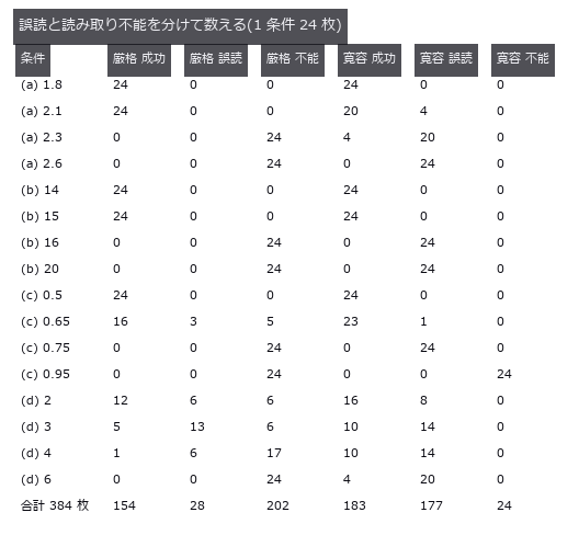
↑ Where a 1-D Barcode Stops Reading — Counting Misreads and Unreadables Separately ―― A home-made simple code (not a real standard) damaged four ways, with success, misread and unreadable counted as three separate outcomes. Over the 384 images past the onset of damage, the strict decoder that checks run structure misreads 7.3 %, while the lenient decoder that always returns nine digits misreads 46.1 % — and has the higher success rate (47.7 % versus 40.1 %). The tilt cliff is pure geometry (predicted 15.95 degrees) and lands between 15 and 16 degrees.
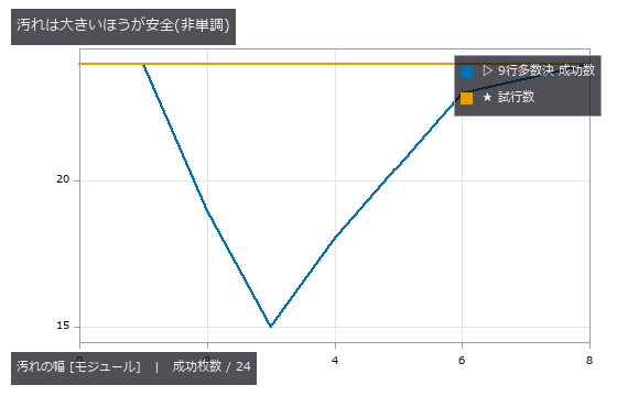
↑ The measurement ―― 小さい汚れは行が「読めてしまう」ので誤った票を投じる。大きい汚れは棄権するので多数決が効く。 (figure labels are in Japanese; the numbers are the same)
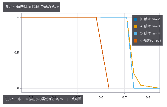
↑ ぼけ 3 本(m=2,3,4 px)は 1 本に重なる。
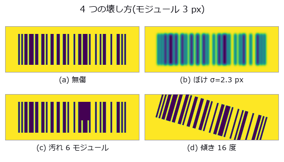
↑ (d) は走査線が符号の上下からはみ出す角度。
py -3.11 examples/poc_barcode_1d.py
Source: examples/poc_barcode_1d.py
This run produced 4 figures in total - see them all
Ops used (notes): decode_barcode · gen_measure_rectangle2 · measure_pos · vol_edge_probe
No.2026.093 —— Electrode tortuosity from CT — the rule of thumb only sees porosity
On a synthetic micro-CT particle bed, Bruggeman is compared with a numerical reference from steady-state diffusion on the same binary volume under stated boundary conditions. For this family eps=0.4448 gives 1.499 versus 1.843 (-18.6%); sweeping 0.691 to 0.168 grows error -8.2% to -69.1%, with fitted exponents 1.78/2.70. Flattening particles 4:1 raises through-plane tau 1.843 to 6.794 while the rule stays near 1.5. Closed pores reach 1.92% and cannot explain the sweep alone; narrow necks are a candidate without isolated causality. Straight pores give numerical tau=1 versus Bruggeman 2; disconnected pores return no_through_path.
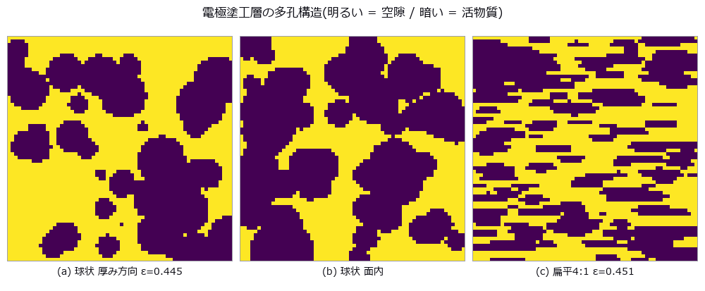
↑ Electrode tortuosity from CT — the rule of thumb only sees porosity ―― On a synthetic micro-CT particle bed, Bruggeman is compared with a numerical reference from steady-state diffusion on the same binary volume under stated boundary conditions. For this family eps=0.4448 gives 1.499 versus 1.843 (-18.6%); sweeping 0.691 to 0.168 grows error -8.2% to -69.1%, with fitted exponents 1.78/2.70. Flattening particles 4:1 raises through-plane tau 1.843 to 6.794 while the rule stays near 1.5. Closed pores reach 1.92% and cannot explain the sweep alone; narrow necks are a candidate without isolated causality. Straight pores give numerical tau=1 versus Bruggeman 2; disconnected pores return no_through_path.
Terms: Bruggeman — An effective-medium relation that approximates transport in a porous material by a power of porosity, often used as a baseline for tortuosity or effective diffusivity.

↑ The measurement ―― 左: 上端 1 / 下端 0 の濃度場。等濃度線が固相を避けて曲がる分が遠回り。右: bond ごとの散逸(明るいほど流れが集中している = 首)。 (figure labels are in Japanese; the numbers are the same)

↑ ε が下がるほど経験則と真値が開く。

↑ この回の図
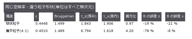
↑ 経験則は向きを持てない。
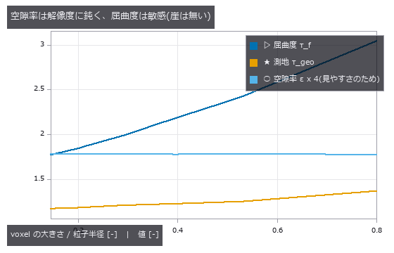
↑ 同じ物理構造を粗い格子から細かい格子まで。
py -3.11 examples/poc_battery_electrode_tortuosity.py
Source: examples/poc_battery_electrode_tortuosity.py
This run produced 6 figures in total - see them all
Ops used (notes): intersection · vol_distance_transform · vol_label
No.2026.004 —— Seven-Level SNR Sweep on Synthetic Bearing Signals — Raw versus Envelope Detection Rates
Bearing diagnosis needs a limit for finding fault impacts inside noise. A known impulse train was buried until the amplitude trace still detected every trial at -18.4 dB SNR. This processing reaches deeper than raw frequencies, but produces false alarms unless its cutoff comes from fault-free records.
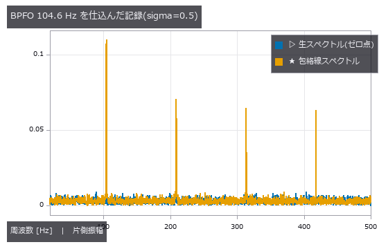
↑ Seven-Level SNR Sweep on Synthetic Bearing Signals — Raw versus Envelope Detection Rates ―― A synthetic impulse train at closed-form BPFO 104.556 Hz is tested at seven SNR levels with ten seeds each. The lowest 10/10 points are -0.9 dB raw and -18.4 dB envelope (17.5 dB apart), empirical coarse-grid points rather than detection limits. Even 10/10 gives a 74.1% one-sided 95% lower bound. On 20 null records independent of threshold selection, false alarms are 0/20 with a 13.9% one-sided 95% upper bound.
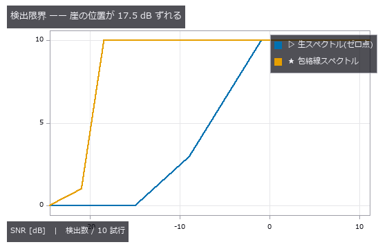
↑ The measurement ―― どちらも最悪条件では 0 に落ちる。包絡線は万能ではなく、崖が悪い SNR 側へ動くだけ。 (figure labels are in Japanese; the numbers are the same)
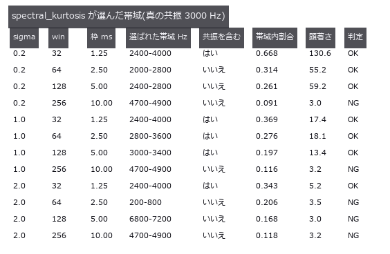
↑ win=32 は毎回共振を含み、win=256 は毎回外す。
py -3.11 examples/poc_bearing_diagnosis.py
Source: examples/poc_bearing_diagnosis.py
This run produced 3 figures in total - see them all
Ops used (notes): bearing_defect_frequencies · envelope_spectrum · spectral_kurtosis · spectrum · synthesize_bearing_signal
No.2026.094 —— Bump coplanarity versus substrate warpage — subtract too much and the real defect goes with it
Warpage removal can absorb a genuinely low bump into the correction surface. Curves fitted to a seeded pillar field left a 1.23 µm readout error after quadratic correction. Raising the order does not help, and a broad low-order defect vanishes into reported warpage while missed bumps increase.
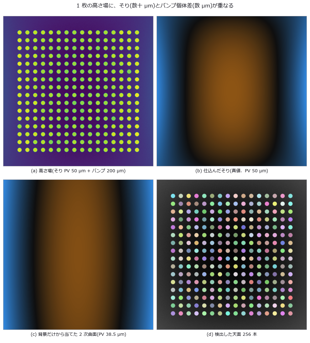
↑ Bump coplanarity versus substrate warpage — subtract too much and the real defect goes with it ―― A height map of 256 Cu pillars is planted with 50 µm PV warpage, 4 µm 1-sigma pillar-to-pillar spread and six short bumps. The zero point — subtract only a least-squares plane, the JEDEC seating plane — reads the individual deviation with 8.84 µm RMS error (2.2x the real spread), raising 58 false rejects while missing one genuinely short bump. A quadratic reference surface brings it to 1.23 µm with zero false rejects; a cubic one is worse (1.37 µm), because the planted high-order mode is quartic and the four extra terms only absorb real signal. The cliff is predictable from geometry: the quadratic fit degrades to the 4 µm level at 169.9 µm PV (predicted) versus 169.4 µm (measured). Adding a real low-order defect — the centre sagging 8 µm — removes 88.2 % of it from the residual while the short-bump detection count stays at 5 of 6, and misses rise from 0 to 2; the lost signal reappears as warpage growing 30.06 to 36.20 µm.
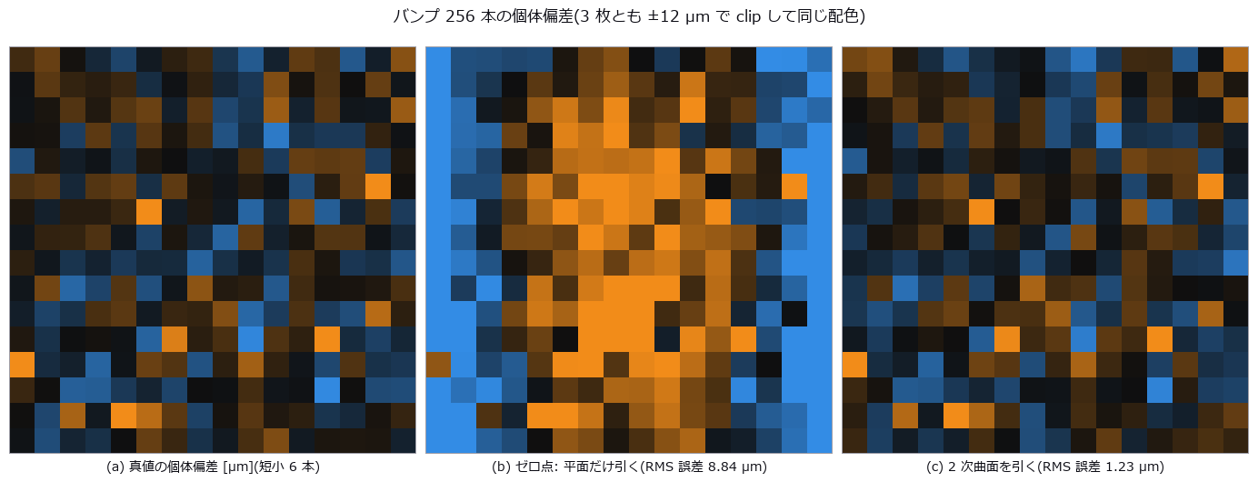
↑ The measurement (figure labels are in Japanese; the numbers are the same)
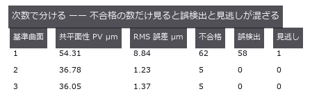
↑ 真値の共平面性は 38.44 µm、本当に仕様外なのは 5 本。

↑ 左端の 6 本が仕込んだ短小。
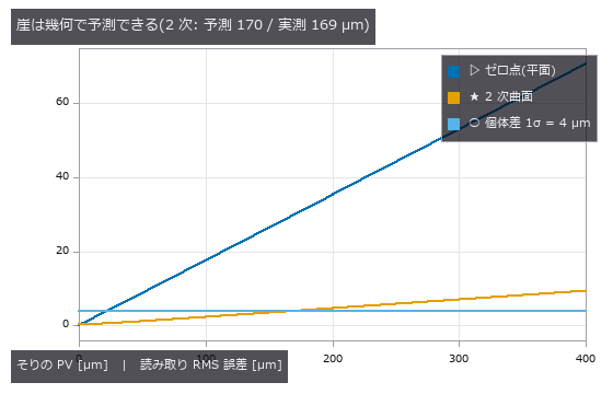
↑ そりの形を固定すれば、取り切れない残りは PV に比例する。

↑ 消えた分はそり側の数字に足されている(+6.14 µm)。
py -3.11 examples/poc_bump_coplanarity.py
Source: examples/poc_bump_coplanarity.py
This run produced 6 figures in total - see them all
Ops used (notes): auto_threshold · background_flatten · blob_features · blob_label · blob_overlay · eval_poly_surface · fit_poly_surface · surface_form_error
No.2026.009 —— Concrete Crack Width Is Thinner Than a Pixel — Counting Width Versus Integrating Width
Cracks from 0.05 to 2.0 mm wide in a field where 1 px = 0.20 mm, measured by thresholding-and-counting and by integrating the intensity deficit across the crack. Thresholding returns nothing at or below 0.20 mm and reports 0.200 mm for all four true widths between 0.25 and 0.40 mm. Integration tracks continuously down to 0.05 mm (0.25 px), but curved illumination adds a +0.1741 mm offset under a first-order baseline (+0.0062 mm with second order).
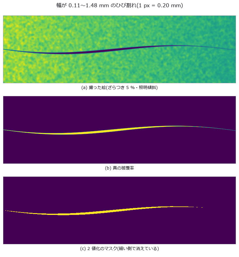
↑ Concrete Crack Width Is Thinner Than a Pixel — Counting Width Versus Integrating Width ―― Cracks from 0.05 to 2.0 mm wide in a field where 1 px = 0.20 mm, measured by thresholding-and-counting and by integrating the intensity deficit across the crack. Thresholding returns nothing at or below 0.20 mm and reports 0.200 mm for all four true widths between 0.25 and 0.40 mm. Integration tracks continuously down to 0.05 mm (0.25 px), but curved illumination adds a +0.1741 mm offset under a first-order baseline (+0.0062 mm with second order).
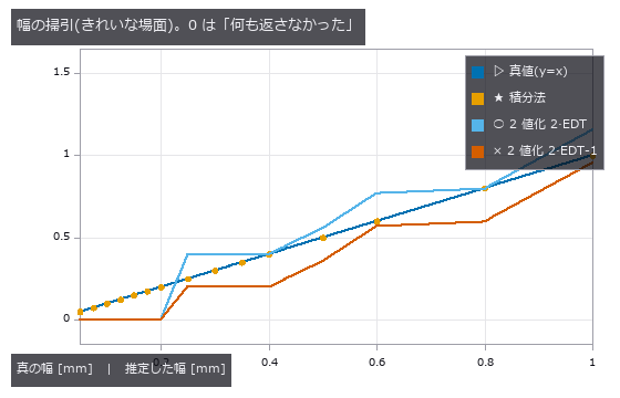
↑ The measurement ―― 2 値化の 2 本は階段。0.20 mm(1 px)以下ではマスクが空になり 0(= 未検出)へ落ちる。積分法は 0.05 mm (0.25 px)まで直線 y=x に乗る。 (figure labels are in Japanese; the numbers are the same)
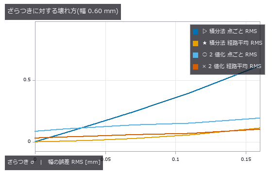
↑ 点ごとでは 2 値化が下に見えるが、経路平均に直すと積分法の散らばりは消え、2 値化の偏りは残る。
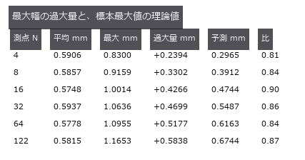
↑ 真の幅は 0.60 mm 固定。
py -3.11 examples/poc_crack_width.py
Source: examples/poc_crack_width.py
This run produced 4 figures in total - see them all
Ops used (notes): distance_transform · sk_medial · skeleton · thinning · vol_distance_transform
No.2026.017 —— Defects Buried in a Periodic Background — What a Pooled ROC (true-positive versus false-positive curve) Hides
Three defect classes (thread break, stain, dim patch) buried in a weave of period 8 px, with the detector’s score map and per-class ROC (true-positive versus false-positive curve) curves side by side. The everyday recipe ‘notch out the grid, remove low frequencies’ pools to an AUC of 0.8113 and looks like a pass, but the dim-patch class alone scores 0.4746, worse than chance. The one line that removes low frequencies was deleting the defect along with the lighting; drop it and the class recovers to 0.9998.
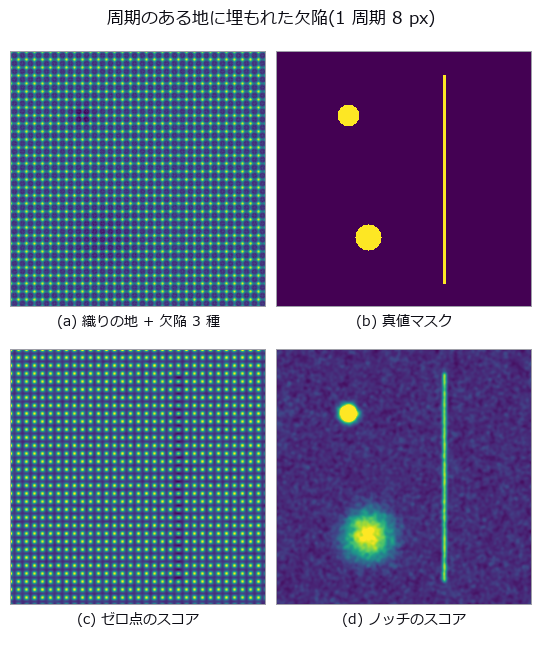
↑ Defects Buried in a Periodic Background — What a Pooled ROC (true-positive versus false-positive curve) Hides ―― Three defect classes (thread break, stain, dim patch) buried in a weave of period 8 px, with the detector’s score map and per-class ROC (true-positive versus false-positive curve) curves side by side. The everyday recipe ‘notch out the grid, remove low frequencies’ pools to an AUC of 0.8113 and looks like a pass, but the dim-patch class alone scores 0.4746, worse than chance. The one line that removes low frequencies was deleting the defect along with the lighting; drop it and the class recovers to 0.9998.
Terms: ROC — A curve of true-positive rate against false-positive rate as the decision threshold varies, showing a binary detector’s trade-off.

↑ The measurement (figure labels are in Japanese; the numbers are the same)

↑ 対角線に乗っている系列が盲点。
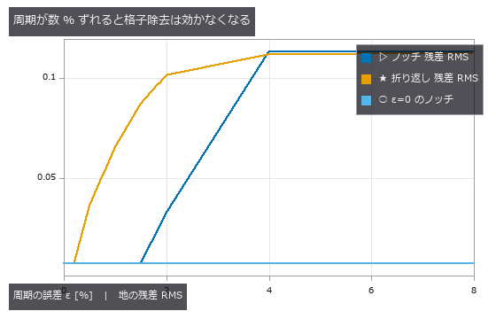
↑ 欠陥の無い地だけで測った残差。
py -3.11 examples/poc_fabric_defect.py
Source: examples/poc_fabric_defect.py
This run produced 4 figures in total - see them all
No.2026.069 —— Digging Where the Sound Says — A Clean Correlation Still Digs in the Wrong Place
Locating a leak in a 120 m buried main from the arrival-time difference at two sensors, with the source, sound speed, attenuation and reflections all planted as ground truth. With the true sound speed the estimate lands within 0.0107 m at 0 dB SNR (1.2x the Knapp-Carter bound of 0.0091 m); the threshold was predicted at -20.1 dB but measured at -12.5 dB, below which the error jumps to 36.0 m — the whole search window. Yet a 10 % error in the assumed sound speed alone moves the dig by 1.798 m (against the predicted (dc/c)(x-L/2) = 1.800 m), and on a pipe that changes from ductile iron to plastic mid-run the time difference is exactly zero, so iron, plastic or their average all miss by 18.001 m: no calibration of a single speed can fix a factor multiplying zero. The reflection prediction failed — GCC-PHAT beat the plain correlation by only 10 %, because 0.121 m of its 0.121 m RMS is bias, and whitening acts on the magnitude while the delay lives in the phase.
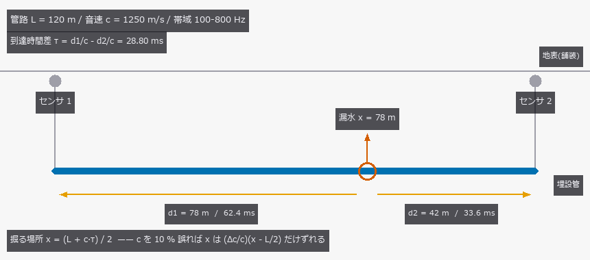
↑ Digging Where the Sound Says — A Clean Correlation Still Digs in the Wrong Place ―― Locating a leak in a 120 m buried main from the arrival-time difference at two sensors, with the source, sound speed, attenuation and reflections all planted as ground truth. With the true sound speed the estimate lands within 0.0107 m at 0 dB SNR (1.2x the Knapp-Carter bound of 0.0091 m); the threshold was predicted at -20.1 dB but measured at -12.5 dB, below which the error jumps to 36.0 m — the whole search window. Yet a 10 % error in the assumed sound speed alone moves the dig by 1.798 m (against the predicted (dc/c)(x-L/2) = 1.800 m), and on a pipe that changes from ductile iron to plastic mid-run the time difference is exactly zero, so iron, plastic or their average all miss by 18.001 m: no calibration of a single speed can fix a factor multiplying zero. The reflection prediction failed — GCC-PHAT beat the plain correlation by only 10 %, because 0.121 m of its 0.121 m RMS is bias, and whitening acts on the magnitude while the delay lives in the phase.
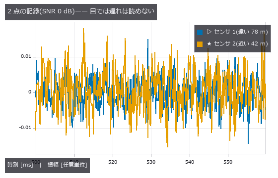
↑ The measurement ―― 同じ漏水源に既知の遅れ 28.80 ms・距離に応じた減衰・独立な広帯域雑音を乗せた。 (figure labels are in Japanese; the numbers are the same)

↑ 探索窓は管路 0-120 m のぶんだけ。
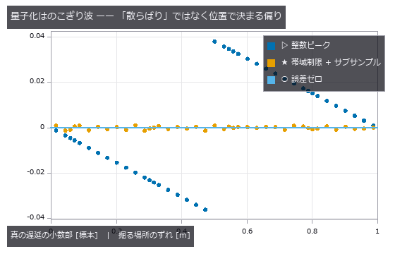
↑ 漏水位置を 41 点振った。
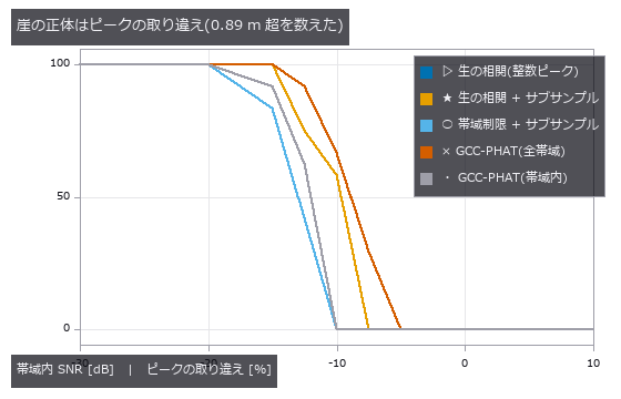
↑ この回の図

↑ 相関の形も相関係数も一切変わらない。
py -3.11 examples/poc_leak_localization.py
Source: examples/poc_leak_localization.py
This run produced 13 figures in total - see them all
Ops used (notes): arrow · bandpass · correlation_score · text_box · transfer_function
No.2026.071 —— Fusing thermal, vibration and geometry for machine health — three sensors, one fact
Six states of a rotating machine (healthy, misalignment, unbalance, outer-race spall, poor lubrication, looseness) are built from closed-form bearing defect frequencies, the exact steady fin-equation solution for the casing temperature, and a planted shaft offset, then classified from three sensors. Fused accuracy is 100.0 % — but vibration alone is also 100.0 %: thermal and geometry add nothing. Misalignment reaches 100.0 % from any single sensor (correlations with the true severity 0.843 / 0.841 / 0.978 — three faces of one number), while thermal alone can never separate healthy, unbalance and looseness (48/48 confusions inside that trio) and dropping vibration takes them from 100.0 % to 50.0 % / 31.2 %. Fusion only earns its keep once vibration breaks: at noise sigma 1.6 it lifts 45.8 % to 78.1 %. The cliffs were predicted on single features: the 0.5X order bin needs T > 2/f_r = 68.6 ms (measured d’ 2.45 -> 4.32 across the 50 -> 70 ms step), the thermal spread dies past the 66 mm half-diameter (d’ 0.00 at 96 mm pitch). The sideband prediction 1/T < FTF = 86.1 ms was wrong; the peak-reading window condition 1.2/FTF = 103 ms is the right one.
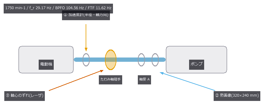
↑ Fusing thermal, vibration and geometry for machine health — three sensors, one fact ―― Six states of a rotating machine (healthy, misalignment, unbalance, outer-race spall, poor lubrication, looseness) are built from closed-form bearing defect frequencies, the exact steady fin-equation solution for the casing temperature, and a planted shaft offset, then classified from three sensors. Fused accuracy is 100.0 % — but vibration alone is also 100.0 %: thermal and geometry add nothing. Misalignment reaches 100.0 % from any single sensor (correlations with the true severity 0.843 / 0.841 / 0.978 — three faces of one number), while thermal alone can never separate healthy, unbalance and looseness (48/48 confusions inside that trio) and dropping vibration takes them from 100.0 % to 50.0 % / 31.2 %. Fusion only earns its keep once vibration breaks: at noise sigma 1.6 it lifts 45.8 % to 78.1 %. The cliffs were predicted on single features: the 0.5X order bin needs T > 2/f_r = 68.6 ms (measured d’ 2.45 -> 4.32 across the 50 -> 70 ms step), the thermal spread dies past the 66 mm half-diameter (d’ 0.00 at 96 mm pitch). The sideband prediction 1/T < FTF = 86.1 ms was wrong; the peak-reading window condition 1.2/FTF = 103 ms is the right one.
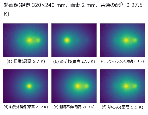
↑ The measurement ―― 軸受外輪傷は狭く熱く、潤滑不良は広く熱い。最高温度だけ見ると同じ顔になる。 (figure labels are in Japanese; the numbers are the same)

↑ 芯ずれは 2X、アンバランスは 1X、ゆるみは 0.5X と櫛。
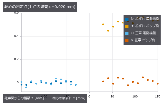
↑ 平行ずれ(切片)と角度ずれ(傾き)を fit_line3 で分けて取る。

↑ 芯ずれと軸受外輪傷は無傷。

↑ 予測は 68.6 ms(0.5X の次数ビン)と 86.1 ms(FTF 側帯波)。
py -3.11 examples/poc_machine_condition_fusion.py
Source: examples/poc_machine_condition_fusion.py
This run produced 13 figures in total - see them all
Ops used (notes): angle_between_lines · arrow · bearing_defect_frequencies · blob_label · distance_point_line · ellipse · fuse · jitter · mat_pinv · rounded_rect · spectrum · stat_correlation · synthesize_bearing_signal · text_box
No.2026.024 —— Reading a Binary Matrix Code — Geometry Always Dies First
A code with QR-style layout and random data bits (no error correction), damaged by blur, tilt and occlusion, with the raw bit error rate counted directly. The nulls sit at chance (0.526 / 0.507) while the reader scores 0.0000. Cliffs: 78 degrees of tilt, two modules of finder-pattern occlusion; run beside the condition that receives the true homography, localisation is always the stage that fails first.

↑ Reading a Binary Matrix Code — Geometry Always Dies First ―― A code with QR-style layout and random data bits (no error correction), damaged by blur, tilt and occlusion, with the raw bit error rate counted directly. The nulls sit at chance (0.526 / 0.507) while the reader scores 0.0000. Cliffs: 78 degrees of tilt, two modules of finder-pattern occlusion; run beside the condition that receives the true homography, localisation is always the stage that fails first.
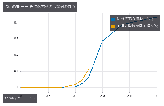
↑ The measurement ―― 自力検出の線は sigma/m 0.50 を最後に途切れる(0.60 では位置検出パターンが見つからない)。標本化はそこでまだ BER 0.07 で読めている。 (figure labels are in Japanese; the numbers are the same)
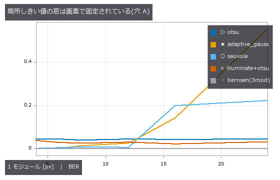
↑ 照明ムラ 0.9 固定。
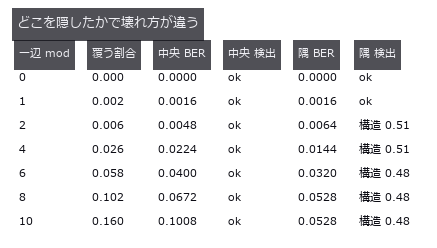
↑ 位置検出パターンは一辺 2 モジュール(全体の 0.6 %)で致命的。
py -3.11 examples/poc_matrix_code_reading.py
Source: examples/poc_matrix_code_reading.py
This run produced 4 figures in total - see them all
Ops used (notes): adaptive_gauss_thresh · corner_response · illuminate · image_to_world_plane · otsu · sk_sauvola
No.2026.025 —— Can Display-Inspection Moire (beat fringe between periodic patterns) Be Told From Real Non-Uniformity?
Moire (beat fringe between periodic patterns) from the interference of the display’s stripes with the camera’s pixel grid, overlaid on genuine luminance non-uniformity in one image. At a smoothing σ of 8 px the total error is +0.9 %, made of +8.3 % moire leakage cancelling -7.4 % attenuation of the real defect. At k = 0.67 the fundamental beat looks safe, yet the third harmonic lands in the defect band and the leakage reaches +202.6 % of the true value.
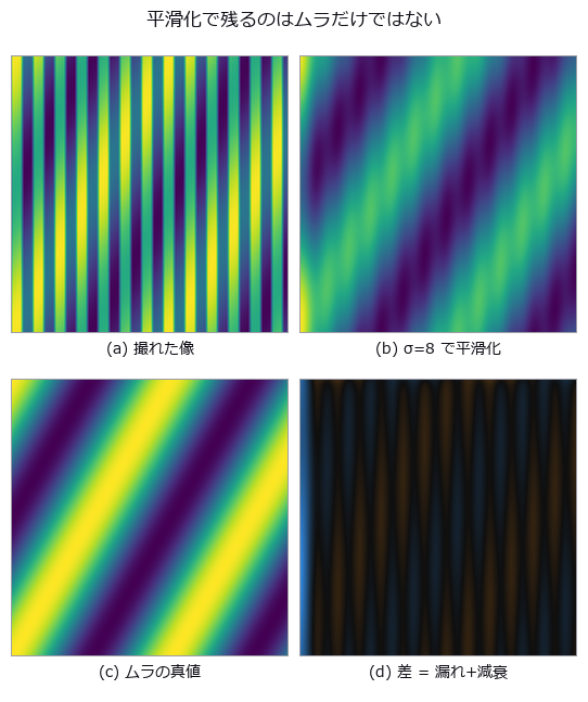
↑ Can Display-Inspection Moire (beat fringe between periodic patterns) Be Told From Real Non-Uniformity? ―― Moire (beat fringe between periodic patterns) from the interference of the display’s stripes with the camera’s pixel grid, overlaid on genuine luminance non-uniformity in one image. At a smoothing σ of 8 px the total error is +0.9 %, made of +8.3 % moire leakage cancelling -7.4 % attenuation of the real defect. At k = 0.67 the fundamental beat looks safe, yet the third harmonic lands in the defect band and the leakage reaches +202.6 % of the true value.
Terms: Moiré — A long-period fringe produced at the difference spatial frequency when two patterns with slightly different pitch or orientation are superposed.
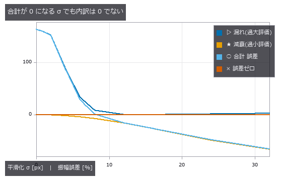
↑ The measurement ―― σ≈8 px で漏れと減衰が釣り合う。合計だけ見ると「良い測り方」に見える。 (figure labels are in Japanese; the numbers are the same)
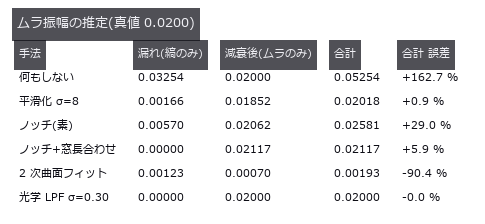
↑ この回の図
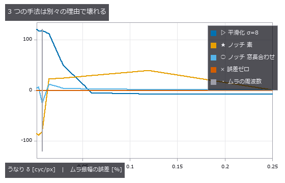
↑ 縦線がムラの周波数。
py -3.11 examples/poc_moire_screen.py
Source: examples/poc_moire_screen.py
This run produced 4 figures in total - see them all
Ops used (notes): background_flatten · fft_image · gauss_image · halftone_moire_period · lattice_moire_peak · moire_differential_shift · moire_magnification · moire_mark_read · moire_overlay_image · moire_phase · moire_phase_crlb · moire_phase_to_shift · moire_talbot_gap · reflect
No.2026.102 —— Print Misregistration from the Sheet — A Halftone Is a Lattice, So the Answer Is Not Unique
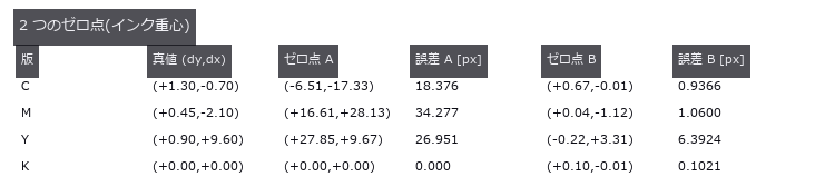
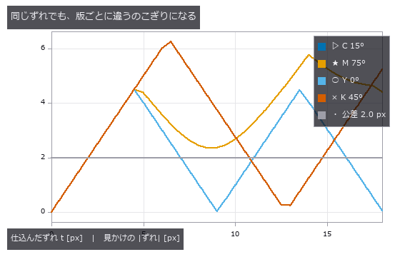
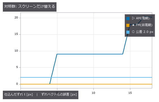
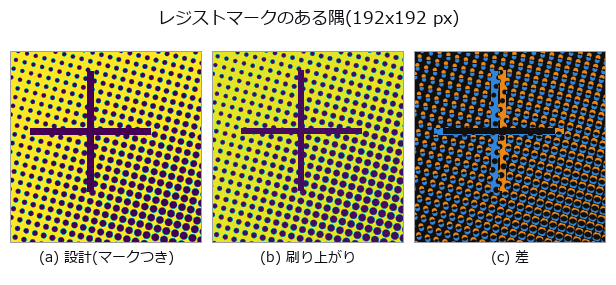
Measuring print misregistration from the printed sheet. Four CMYK plates carry the conventional screen angles (C 15, M 75, Y 0, K 45 degrees) at 133 lpi scanned at 1200 dpi, giving a screen pitch of 9.02 px, and each plate is displaced by a known amount. The central claim is geometry: a halftone is a lattice, so correlation recovers not the displacement d but d modulo the screen lattice. Along the lattice axes that limit is p/2 = 4.51 px and along the diagonal p/sqrt(2) = 6.38 px; beyond it the measurement folds back. Stated in closed form before measuring, it matches at 144 of 148 points (four plates by 37 sweep positions) to within 0.1096 px. The four exceptions are ties on the boundary of the fundamental cell, with at most 0.165 px of margin, and reducing modulo the lattice makes every point agree: the estimator is not wrong, it returns one of the lattice-equivalent answers, and two independent estimators fold identically. The consequence is concrete. A true displacement of 9.64 px, 4.8 times the 2.0 px tolerance, appears as 1.09 to 3.32 px depending only on the screen angle, so two of the four plates look like they pass — from one sheet displaced by one amount. The null baseline, the centroid of ink, does not fold but loses its scale: the slope follows the closed form k = 1 - beta, where beta is the ink of the flat background over the total ink, predicted 0.3983 against 0.3711 measured. One effect was not predicted at all: a 0.9864 px ripple at the screen pitch, caused by rows of dots entering and leaving at the window edge, which a tapered-window control drops to 0.0048 px. Switching to an FM (stochastic) screen removes the folding entirely, with an error of at most 0.0029 px across the whole sweep, which places the blame on the periodicity of the AM screen rather than on the estimator, at the cost of 0.91 times the contrast. A window containing a registration mark reads correctly to 0.0823 px, but with 0.600 % paper stretch and 0.120 degrees of plate rotation the error grows linearly with distance at 0.006319 px per px and exceeds tolerance from 316.5 px predicted, 322.5 px measured — 44 % of the sheet. Two rulers reverse the ranking: raw correlation is the most accurate at 0.0071 px yet agrees with the pass/fail verdict only 67.6 % of the time, while low-pass filtering agrees 89.2 % of the time at 94 times the error; a two-stage estimator that picks the representative with the blunt method and refines with the sharp one wins both, and it fails exactly at the points where the coarse error exceeded the cell radius of 4.511 px. The synthesiser itself was a trap: at 150 lpi and 1200 dpi the pitch is exactly 8.00 px, every dot samples in phase, and the centroid jumps 1.4 px for each 0.5 px of displacement — avoiding the integer ratio is the fix, not supersampling. Finally, an operator used outside its domain failed confidently: fs.frame_align returned inlier_ratio 1.00 and rms_px 0.645 while missing the true (0.00, +1.30) by 80.85 px, and the answer was not even a lattice vector. That finding was fixed in the operator: its docstring now records the measurement, and the vote histogram’s runner-up over winner is returned as vote_margin — 1.000 on this halftone against 0.143 on a star field, where the agreement ratio is 1.00 in both.
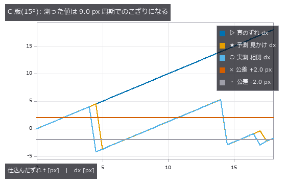
↑ Print Misregistration from the Sheet — A Halftone Is a Lattice, So the Answer Is Not Unique ―― Measuring print misregistration from the printed sheet. Four CMYK plates carry the conventional screen angles (C 15, M 75, Y 0, K 45 degrees) at 133 lpi scanned at 1200 dpi, giving a screen pitch of 9.02 px, and each plate is displaced by a known amount. The central claim is geometry: a halftone is a lattice, so correlation recovers not the displacement d but d modulo the screen lattice. Along the lattice axes that limit is p/2 = 4.51 px and along the diagonal p/sqrt(2) = 6.38 px; beyond it the measurement folds back. Stated in closed form before measuring, it matches at 144 of 148 points (four plates by 37 sweep positions) to within 0.1096 px. The four exceptions are ties on the boundary of the fundamental cell, with at most 0.165 px of margin, and reducing modulo the lattice makes every point agree: the estimator is not wrong, it returns one of the lattice-equivalent answers, and two independent estimators fold identically. The consequence is concrete. A true displacement of 9.64 px, 4.8 times the 2.0 px tolerance, appears as 1.09 to 3.32 px depending only on the screen angle, so two of the four plates look like they pass — from one sheet displaced by one amount. The null baseline, the centroid of ink, does not fold but loses its scale: the slope follows the closed form k = 1 - beta, where beta is the ink of the flat background over the total ink, predicted 0.3983 against 0.3711 measured. One effect was not predicted at all: a 0.9864 px ripple at the screen pitch, caused by rows of dots entering and leaving at the window edge, which a tapered-window control drops to 0.0048 px. Switching to an FM (stochastic) screen removes the folding entirely, with an error of at most 0.0029 px across the whole sweep, which places the blame on the periodicity of the AM screen rather than on the estimator, at the cost of 0.91 times the contrast. A window containing a registration mark reads correctly to 0.0823 px, but with 0.600 % paper stretch and 0.120 degrees of plate rotation the error grows linearly with distance at 0.006319 px per px and exceeds tolerance from 316.5 px predicted, 322.5 px measured — 44 % of the sheet. Two rulers reverse the ranking: raw correlation is the most accurate at 0.0071 px yet agrees with the pass/fail verdict only 67.6 % of the time, while low-pass filtering agrees 89.2 % of the time at 94 times the error; a two-stage estimator that picks the representative with the blunt method and refines with the sharp one wins both, and it fails exactly at the points where the coarse error exceeded the cell radius of 4.511 px. The synthesiser itself was a trap: at 150 lpi and 1200 dpi the pitch is exactly 8.00 px, every dot samples in phase, and the centroid jumps 1.4 px for each 0.5 px of displacement — avoiding the integer ratio is the fix, not supersampling. Finally, an operator used outside its domain failed confidently: fs.frame_align returned inlier_ratio 1.00 and rms_px 0.645 while missing the true (0.00, +1.30) by 80.85 px, and the answer was not even a lattice vector. That finding was fixed in the operator: its docstring now records the measurement, and the vote histogram’s runner-up over winner is returned as vote_margin — 1.000 on this halftone against 0.143 on a star field, where the agreement ratio is 1.00 in both.
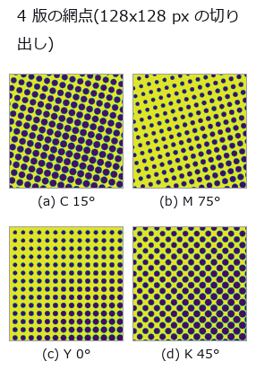
↑ The measurement ―― スクリーン角が違うので格子の向きが違う。ピッチはどれも 9.02 px。同じ物理的なずれでも、この格子の違いが「見かけのずれ」を版ごとに変える(5 節) (figure labels are in Japanese; the numbers are the same)
↑ この回の図
↑ スクリーン角が違えば格子も違う。
↑ 絵柄も推定器も同じ。
↑ 十字は非周期なので相関のピークが 1 つに決まる。
py -3.11 examples/poc_print_registration.py
Source: examples/poc_print_registration.py
This run produced 13 figures in total - see them all
Ops used (notes): fly_hex_lattice · fly_vogel_lattice · frame_align · halftone_moire_period · halftone_screen · lattice_moire_peak · peak_subbin · piv_cross_correlate
No.2026.116 —— How Faint a Defect Can Still Be Found — Planting a Known Truth in a Real Background
The usual way to estimate “how faint a defect can we still catch” is to measure the limit on a synthetic image: a flat field plus white noise. This exhibit measures how optimistic that estimate is, while keeping an exact ground truth. The backgrounds are three CC0 photographs (brick / grass / gravel); what is planted into them is a Gaussian defect of known position, width and amplitude. The control is a synthetic field whose residual sigma — the variation the detector actually sees — is matched to the real one, so the amount of noise is equal and only structure differs. The verdict is the smallest amplitude at which the planted position becomes the peak of the response; no threshold is involved, so per-image normalisation inside an operator cannot skew it. Matching the noise is not enough: the real backgrounds raise the floor by 2.03x to 3.47x. What sets the floor is structure, not noise. The gap survives all 18 knob settings (three background windows x two defect sizes x three grounds, 1.72x-4.56x) and both detectors — a matched filter and fullseye’s laplace_of_gauss. A prediction that failed: “the gap widens for larger defects” turned out to be an artefact of the amplitude grid — on 34 steps the two sizes round to different grid points, on 60 steps both land at 3.30x. The grid is a knob too. “Real data is position-dependent” is also wrong: the spread of the floor across positions is 16.8x on brick but 2.4x on grass and 3.3x on gravel, indistinguishable from the 3.3x of the matched synthetic control. What creates the spread is the mortar lattice — a structure — not the fact that the image is a photograph. And the null model wins on a single metric. Taking the brightest raw pixel, with no background removed, localises the defect at 0.65x-0.90x the amplitude the matched filter needs, because the matched filter amplifies the background’s structure too; false alarms on a defect-free surface tie at 0 on brick. The two separate the moment the lamp drifts by 2 %: the null model fires 10.3 times per 10,000 pixels while the matched filter stays at 0.0, because a raw-pixel threshold is an absolute brightness. Count localisation, false alarms and drift separately, or a useless detector can be made to win.

↑ How Faint a Defect Can Still Be Found — Planting a Known Truth in a Real Background ―― The usual way to estimate “how faint a defect can we still catch” is to measure the limit on a synthetic image: a flat field plus white noise. This exhibit measures how optimistic that estimate is, while keeping an exact ground truth. The backgrounds are three CC0 photographs (brick / grass / gravel); what is planted into them is a Gaussian defect of known position, width and amplitude. The control is a synthetic field whose residual sigma — the variation the detector actually sees — is matched to the real one, so the amount of noise is equal and only structure differs. The verdict is the smallest amplitude at which the planted position becomes the peak of the response; no threshold is involved, so per-image normalisation inside an operator cannot skew it. Matching the noise is not enough: the real backgrounds raise the floor by 2.03x to 3.47x. What sets the floor is structure, not noise. The gap survives all 18 knob settings (three background windows x two defect sizes x three grounds, 1.72x-4.56x) and both detectors — a matched filter and fullseye’s laplace_of_gauss. A prediction that failed: “the gap widens for larger defects” turned out to be an artefact of the amplitude grid — on 34 steps the two sizes round to different grid points, on 60 steps both land at 3.30x. The grid is a knob too. “Real data is position-dependent” is also wrong: the spread of the floor across positions is 16.8x on brick but 2.4x on grass and 3.3x on gravel, indistinguishable from the 3.3x of the matched synthetic control. What creates the spread is the mortar lattice — a structure — not the fact that the image is a photograph. And the null model wins on a single metric. Taking the brightest raw pixel, with no background removed, localises the defect at 0.65x-0.90x the amplitude the matched filter needs, because the matched filter amplifies the background’s structure too; false alarms on a defect-free surface tie at 0 on brick. The two separate the moment the lamp drifts by 2 %: the null model fires 10.3 times per 10,000 pixels while the matched filter stays at 0.0, because a raw-pixel threshold is an absolute brightness. Count localisation, false alarms and drift separately, or a useless detector can be made to win.
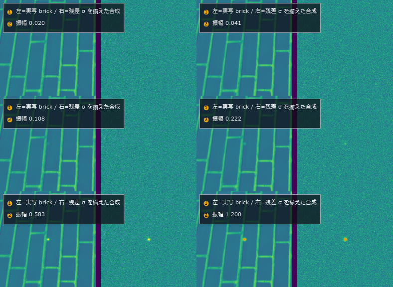
↑ The measurement ―― 同じ欠陥を振幅 0.02 から 1.20 まで上げていく。左=実写の brick、右=残差 σ を揃えた合成の地。雑音の量は同じなのに、右のほうが先に見えてくる。 (figure labels are in Japanese; the numbers are the same)
py -3.11 examples/poc_real_defect_floor.py
Source: examples/poc_real_defect_floor.py
This run produced 2 figures in total - see them all
Ops used (notes): annotate_inset · annotate_legend · laplace_of_gauss · reflect
No.2026.109 —— Rotating Real Textures — Rotation Invariance Holds Only Where It Is Not Needed
Three real textures (brick, grass, gravel, all CC0) rotated by known angles, measuring how far the descriptor drifts from itself. The benchmark is set before measuring: the smallest distance between materials, 0.01250 between grass and gravel, is the resolution of the task, and any rotation drift beyond it means a rotated sample is further from itself than from a different material. The anisotropic brick drifts 0.0433 at five degrees and 0.1205 at sixty, 9.6 times the resolution, while grass and gravel stay at 0.0005 to 0.0024, effectively invariant. Two controls isolate the cause: interpolation alone, measured by rotating plus seven and back minus seven degrees, contributes 0.03685 for brick, and an exact ninety-degree rotation with no interpolation at all still gives 0.08501, or 6.8 times the resolution. Anisotropy can be measured independently and explains the ranking: the global concentration of gradient orientation is 0.309 for brick against 0.027 and 0.029 for the others. Switching to rotation-invariant encodings brings brick from 9.64 down through 5.49 to 1.72 — never below one — while the isotropic pair improves tenfold, from 0.17 to 0.02. LBP’s rotation invariance applies to the cyclic shift of a local pattern; it cannot remove the orientation distribution of the material itself.
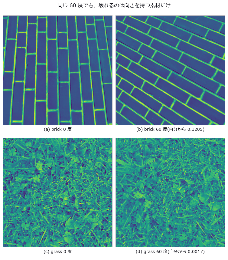
↑ Rotating Real Textures — Rotation Invariance Holds Only Where It Is Not Needed ―― Three real textures (brick, grass, gravel, all CC0) rotated by known angles, measuring how far the descriptor drifts from itself. The benchmark is set before measuring: the smallest distance between materials, 0.01250 between grass and gravel, is the resolution of the task, and any rotation drift beyond it means a rotated sample is further from itself than from a different material. The anisotropic brick drifts 0.0433 at five degrees and 0.1205 at sixty, 9.6 times the resolution, while grass and gravel stay at 0.0005 to 0.0024, effectively invariant. Two controls isolate the cause: interpolation alone, measured by rotating plus seven and back minus seven degrees, contributes 0.03685 for brick, and an exact ninety-degree rotation with no interpolation at all still gives 0.08501, or 6.8 times the resolution. Anisotropy can be measured independently and explains the ranking: the global concentration of gradient orientation is 0.309 for brick against 0.027 and 0.029 for the others. Switching to rotation-invariant encodings brings brick from 9.64 down through 5.49 to 1.72 — never below one — while the isotropic pair improves tenfold, from 0.17 to 0.02. LBP’s rotation invariance applies to the cyclic shift of a local pattern; it cannot remove the orientation distribution of the material itself.
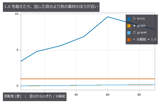
↑ The measurement ―― brick だけが 1 を大きく超える(最大 9.6 倍)。 (figure labels are in Japanese; the numbers are the same)
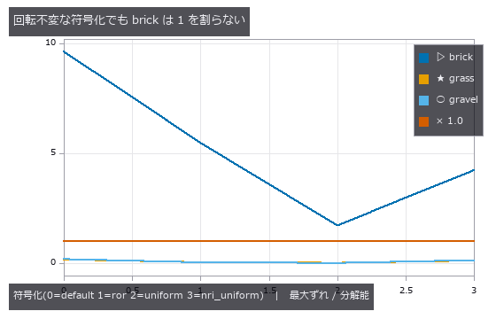
↑ 等方な 2 つは 10 倍良くなる。
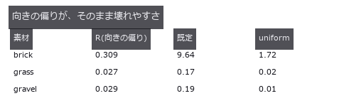
↑ 単位はどれも「分解能に対する比」。
py -3.11 examples/poc_real_texture_invariance.py
Source: examples/poc_real_texture_invariance.py
This run produced 4 figures in total - see them all
Ops used (notes): cooc_feature_matrix · reflect · sk_lbp
No.2026.079 —— Sorting mixed waste by material — what a preprocessor can erase is decided by algebra
Fragments on a belt carry material, dirt, wetness, tilt and occlusion in known amounts, imaged in 64 SWIR (short-wave infrared) bands. Per-fragment degradation is closed form, s(l)=gR(l)exp(-wA_w(l))+(au(l)+c), so invariance can be predicted before measuring: the spectral angle is invariant to the multiplicative g (0.995 to 0.990 as dirt goes 0 to 0.8; 0.993 at 70 degrees of tilt), and a second derivative annihilates the linear baseline (raw SAM falls 0.995 to 0.827 under an additive baseline while the derivative stays at 0.995 at every level). Two predictions failed: wetness is largely removed by the second derivative (0.818 against 0.282 for raw SAM) because a second derivative weights Gaussian bands by 1/sigma^2 ((43/70)^2 = 0.37), and continuum removal beats raw SAM while the baseline is weak (0.983 vs 0.865) but loses once it is strong (0.736 vs 0.827). Featureless metal vanishes under differentiation (recall 0.06) and a flatness gate restores it to 0.98.

↑ Sorting mixed waste by material — what a preprocessor can erase is decided by algebra ―― Fragments on a belt carry material, dirt, wetness, tilt and occlusion in known amounts, imaged in 64 SWIR (short-wave infrared) bands. Per-fragment degradation is closed form, s(l)=gR(l)exp(-wA_w(l))+(au(l)+c), so invariance can be predicted before measuring: the spectral angle is invariant to the multiplicative g (0.995 to 0.990 as dirt goes 0 to 0.8; 0.993 at 70 degrees of tilt), and a second derivative annihilates the linear baseline (raw SAM falls 0.995 to 0.827 under an additive baseline while the derivative stays at 0.995 at every level). Two predictions failed: wetness is largely removed by the second derivative (0.818 against 0.282 for raw SAM) because a second derivative weights Gaussian bands by 1/sigma^2 ((43/70)^2 = 0.37), and continuum removal beats raw SAM while the baseline is weak (0.983 vs 0.865) but loses once it is strong (0.736 vs 0.827). Featureless metal vanishes under differentiation (recall 0.06) and a flatness gate restores it to 0.98.
Terms: SWIR — The short-wave infrared band, roughly around 1 to 3 µm, where material absorption can distinguish objects that look alike in visible light.; SAM — A classifier that compares spectra by the angle between their vectors, making it invariant to a common multiplicative scale.

↑ The measurement ―― PP と PE は骨格が同じ(-CH2-)なのでわざと似せてある。 (figure labels are in Japanese; the numbers are the same)

↑ 乗算汚れ・傾き・重なりは平ら(SAM は明るさに不変)。

↑ この回の図

↑ 1 個の正解率には出ない盲点がここに出る。

↑ この回の図
py -3.11 examples/poc_recycling_sorting.py
Source: examples/poc_recycling_sorting.py
This run produced 14 figures in total - see them all
Ops used (notes): overlay_labels · spectrum
No.2026.084 —— Power loss from solar-cell EL images — dark is not the same as inactive
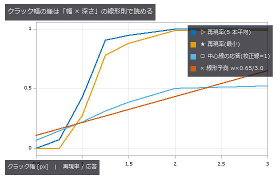
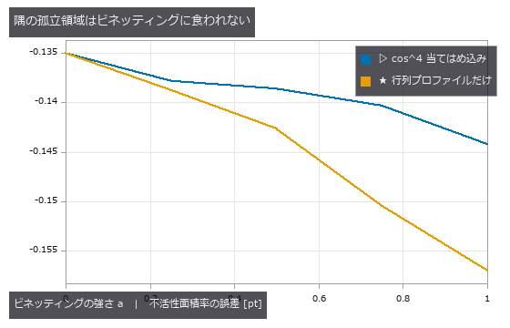
A crystalline-silicon cell (100 fingers, 3 busbars, 70 grains) is rendered in closed form as an EL image with two electrically isolated regions (true inactive area 4.77 %), 5 cracks and 8 finger interruptions, then imaged through cos^4 vignetting and photon noise. The zero-point global threshold reports a dark-pixel fraction of 21.7 % as the inactive area, but 42 % of those pixels are fingers and busbars and 33 % are grains and vignetting; only 20 % are truly inactive. Dividing out the grid with row/column profiles and gating each defect type separately gives 4.61 % (-0.15 points), crack recall 0.88–1.00 and 8/8 interruptions. Because sk_frangi normalises by the per-image maximum, a calibration line only fixes the scale if it is the strongest ridge in the image (a line like the real cracks responds 0.69, a 3 px black line 1.00); without calibration the defect-free cell produces 147 px of false cracks. From grain contrast c=0.24 false cracks and swallowed interruption bands start together, and the crack-width cliff at 1.25 px follows the linear width-times-depth rule (predicted 1.38 px).

↑ Power loss from solar-cell EL images — dark is not the same as inactive ―― A crystalline-silicon cell (100 fingers, 3 busbars, 70 grains) is rendered in closed form as an EL image with two electrically isolated regions (true inactive area 4.77 %), 5 cracks and 8 finger interruptions, then imaged through cos^4 vignetting and photon noise. The zero-point global threshold reports a dark-pixel fraction of 21.7 % as the inactive area, but 42 % of those pixels are fingers and busbars and 33 % are grains and vignetting; only 20 % are truly inactive. Dividing out the grid with row/column profiles and gating each defect type separately gives 4.61 % (-0.15 points), crack recall 0.88–1.00 and 8/8 interruptions. Because sk_frangi normalises by the per-image maximum, a calibration line only fixes the scale if it is the strongest ridge in the image (a line like the real cracks responds 0.69, a 3 px black line 1.00); without calibration the defect-free cell produces 147 px of false cracks. From grain contrast c=0.24 false cracks and swallowed interruption bands start together, and the crack-width cliff at 1.25 px follows the linear width-times-depth rule (predicted 1.38 px).

↑ The measurement (figure labels are in Japanese; the numbers are the same)
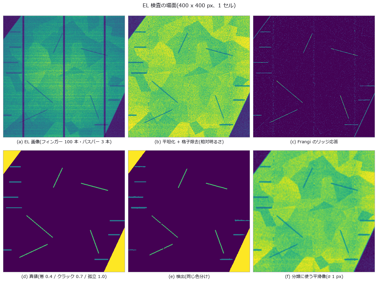
↑ 孤立領域 2 つ・クラック 5 本・断線 8 本。

↑ この回の図
↑ この回の図
↑ この回の図
py -3.11 examples/poc_solar_el_inspection.py
Source: examples/poc_solar_el_inspection.py
This run produced 8 figures in total - see them all
Ops used (notes): aug_vignette · blob_features · blob_label · blob_select · gaussian · gray_closing · hysteresis_threshold · lines_gauss · otsu · sk_frangi · sk_skeleton · total_length · vignette
No.2026.085 —— Solder fillet AOI — three ring lights are a 3-level tilt quantiser, and 70 % of the fillet height sits in the dark
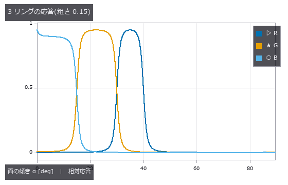
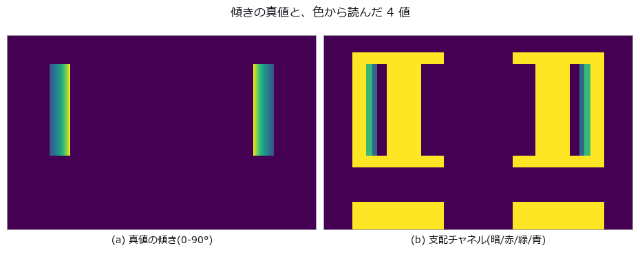
A 1608 chip’s pads and terminations carry circular-arc fillets fixed by contact angle and cross-section area; three ring lights at different elevations (red 30-40°, green 15-30°, blue 0-15° of surface tilt) are integrated over a GGX (microfacet reflection model) lobe to synthesise the AOI image, and joints are graded good / insufficient / bridge / tombstone. With an 18° contact angle the concave arc rises to 72° at the wall, so even the lowest ring sees only 28.8 % of the height (predicted): naively integrating the band tilts recovers 0.284 of the true height. Extrapolating the arc to the wall from the positions where the colour changes lands at +1.7 % ± 5.3 % for free arcs, but once extra solder pins the toe at the pad edge it drifts to -42.3 %. A 0.16 mm placement offset steepens the toe past 30°, the green band vanishes and a good joint is called insufficient although its true height has risen (predicted 0.16 mm; the truth only fails at 0.28 mm). Surface roughness, against expectation, does not move the dark edge; it breaks at roughness 0.5 together with the loss of the red band and at 0.6 the whole fillet drops below the dark threshold. The zero point (Lab distance of the pad mean colour) is 100 % right under reference conditions yet flags 56 % of good joints and 68 % of bridges once offset, roughness and lighting vary — no discrimination — while the arc-based grading scores good 98 % / insufficient 98 % / bridge 100 % / tombstone 88 %, the misses all being lifts of 8.7-11.0°.
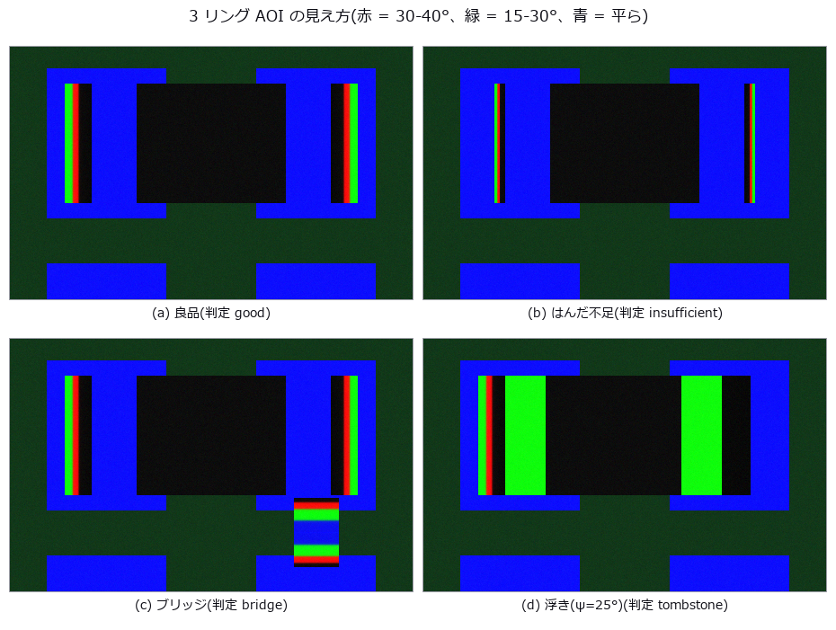
↑ Solder fillet AOI — three ring lights are a 3-level tilt quantiser, and 70 % of the fillet height sits in the dark ―― A 1608 chip’s pads and terminations carry circular-arc fillets fixed by contact angle and cross-section area; three ring lights at different elevations (red 30-40°, green 15-30°, blue 0-15° of surface tilt) are integrated over a GGX (microfacet reflection model) lobe to synthesise the AOI image, and joints are graded good / insufficient / bridge / tombstone. With an 18° contact angle the concave arc rises to 72° at the wall, so even the lowest ring sees only 28.8 % of the height (predicted): naively integrating the band tilts recovers 0.284 of the true height. Extrapolating the arc to the wall from the positions where the colour changes lands at +1.7 % ± 5.3 % for free arcs, but once extra solder pins the toe at the pad edge it drifts to -42.3 %. A 0.16 mm placement offset steepens the toe past 30°, the green band vanishes and a good joint is called insufficient although its true height has risen (predicted 0.16 mm; the truth only fails at 0.28 mm). Surface roughness, against expectation, does not move the dark edge; it breaks at roughness 0.5 together with the loss of the red band and at 0.6 the whole fillet drops below the dark threshold. The zero point (Lab distance of the pad mean colour) is 100 % right under reference conditions yet flags 56 % of good joints and 68 % of bridges once offset, roughness and lighting vary — no discrimination — while the arc-based grading scores good 98 % / insufficient 98 % / bridge 100 % / tombstone 88 %, the misses all being lifts of 8.7-11.0°.
Terms: GGX — A microfacet reflection model using the long-tailed Trowbridge–Reitz distribution of facet normals.
↑ The measurement ―― 鏡面なら窓の端が階段になる。傾き 40° を超えるとどのリングも届かない。 (figure labels are in Japanese; the numbers are the same)
↑ この回の図
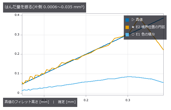
↑ E1 は 0.28 倍の直線に乗る(暗部を見ていない)。
↑ この回の図

↑ この回の図
py -3.11 examples/poc_solder_fillet_aoi.py
Source: examples/poc_solder_fillet_aoi.py
This run produced 12 figures in total - see them all
Ops used (notes): access_channel · blob_features · blob_label · blob_select_largest · brdf_microfacet · illumination_design · intensity · rgb_to_lab · trans_from_rgb
No.2026.121 —— Is the Process in Control, and Is It Capable? — Statistical Process Control from Closed-Form Alone
A series of dimensions and defect counts measured by machine vision, fed through four SPC ops that use no learning at all (each a textbook closed-form with an exact identity to check against). The Xbar-R chart catches a +4σ shift planted at the tail across 4 subgroups at once (n=5 constants A2/D3/D4 = 0.577/0.000/2.115, ISO 8258); CUSUM catches a +0.8σ sustained drift that Shewhart 3σ never flags, at #45 (right after the drift starts). Process capability separates “capable” from “capable at the current centre”: centred on the spec midpoint Cpk = Cp = 1.307, shifted by +1 Cpk = 0.981 < Cp. Multivariate T² folds the simultaneous drift of three correlated measurements into one verdict (UCL from the F-distribution). As with image restoration, a process running and a process in control are measured separately.
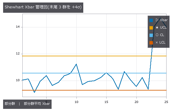
↑ Is the Process in Control, and Is It Capable? — Statistical Process Control from Closed-Form Alone ―― A series of dimensions and defect counts measured by machine vision, fed through four SPC ops that use no learning at all (each a textbook closed-form with an exact identity to check against). The Xbar-R chart catches a +4σ shift planted at the tail across 4 subgroups at once (n=5 constants A2/D3/D4 = 0.577/0.000/2.115, ISO 8258); CUSUM catches a +0.8σ sustained drift that Shewhart 3σ never flags, at #45 (right after the drift starts). Process capability separates “capable” from “capable at the current centre”: centred on the spec midpoint Cpk = Cp = 1.307, shifted by +1 Cpk = 0.981 < Cp. Multivariate T² folds the simultaneous drift of three correlated measurements into one verdict (UCL from the F-distribution). As with image restoration, a process running and a process in control are measured separately.
Terms: Xbar-R — A paired control-chart method that tracks subgroup means and ranges to monitor process location and spread.; CUSUM — A control chart that accumulates deviations from a reference value to detect small sustained shifts in the mean.; Shewhart — A control chart that compares a process statistic with a center line and control limits to flag changes unlikely under common-cause variation.
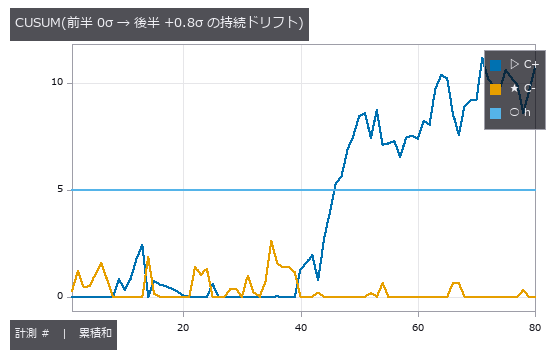
↑ The measurement ―― Shewhart 3σ は 0 件、CUSUM は #46(ドリフト開始の直後)で h=5 を超えて警報。 (figure labels are in Japanese; the numbers are the same)
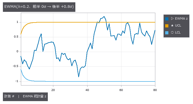
↑ EWMA も #46 で管理限界を越えて警報 —— Shewhart 3σ が見逃す小シフトを CUSUM と同様に捕らえる(限界は最初の数点で漸近値へ広がる)。
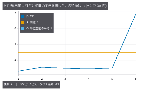
↑ 末尾の行はどの特徴も単独では 3σ 内(当たり 0 件)なのに MD=7.78 —— 正常行の最大 1.10 に対して 7.1 倍。
py -3.11 examples/poc_spc.py
Source: examples/poc_spc.py
This run produced 4 figures in total - see them all
Ops used (notes): spc_capability · spc_cusum · spc_ewma · spc_hotelling_t2 · spc_mt_distance · spc_mt_sn_ratio · spc_mt_unit_space · spc_xbar_r
No.2026.152 —— Every Sensor Reads Normal, Yet the Machine Is Failing — How Much the MT Method Recovers from Univariate 3σ
| The 20 features (vibration, thermal, shape) of the machine-condition PoC: 48 healthy records form a Mahalanobis–Taguchi unit space, and 32 further healthy records set both thresholds — univariate max | z | and MD — at zero false alarms. Healthy machines have strongly correlated features (coupling vs. global temperature: ρ=0.999), so a record that breaks the correlation is far in distance while every single feature stays in range. Of the 169 fault records the univariate rule called “all features normal”, the MT method flags 79 (47 %); the upper-left region of the scatter (left of the univariate threshold, above the MD threshold) is exactly that set. Two exact identities: the unit space’s mean MD² equals (N−1)/N (from the ddof=1 definition), and for two features the point (+z, −z) has MD² = z²/(1−ρ) in closed form. The customary | z | >3 fires by chance 12.5 % of the time with 20 features. Mild faults are a linear blend between normal (0) and fault (1) — the original PoC’s “severity × fault value” produced, at the mild end, a machine quieter and cooler than normal, and detection was not monotone in severity. Synthetic material; the fraction is an upper bound for this correlation structure. |

| *↑ Every Sensor Reads Normal, Yet the Machine Is Failing — How Much the MT Method Recovers from Univariate 3σ ―― The 20 features (vibration, thermal, shape) of the machine-condition PoC: 48 healthy records form a Mahalanobis–Taguchi unit space, and 32 further healthy records set both thresholds — univariate max | z | and MD — at zero false alarms. Healthy machines have strongly correlated features (coupling vs. global temperature: ρ=0.999), so a record that breaks the correlation is far in distance while every single feature stays in range. Of the 169 fault records the univariate rule called “all features normal”, the MT method flags 79 (47 %); the upper-left region of the scatter (left of the univariate threshold, above the MD threshold) is exactly that set. Two exact identities: the unit space’s mean MD² equals (N−1)/N (from the ddof=1 definition), and for two features the point (+z, −z) has MD² = z²/(1−ρ) in closed form. The customary | z | >3 fires by chance 12.5 % of the time with 20 features. Mild faults are a linear blend between normal (0) and fault (1) — the original PoC’s “severity × fault value” produced, at the mild end, a machine quieter and cooler than normal, and detection was not monotone in severity. Synthetic material; the fraction is an upper bound for this correlation structure.* |

↑ The measurement ―― 芯ずれ。差が最大なのは重症度 0.05 で、単変量 25.0 % に対し MT 法 100.0 %。重症度 0.50 以上は両方式とも 100 %。閾値は健全の別標本 32 本で両方式とも誤警報 0。 (figure labels are in Japanese; the numbers are the same)

↑ アンバランス。

↑ 軸受外輪傷。

↑ 潤滑不良。

↑ ゆるみ。
py -3.11 examples/poc_mt_hidden_fault.py
Source: examples/poc_mt_hidden_fault.py
This run produced 6 figures in total - see them all
Ops used (notes): spc_mt_distance · spc_mt_unit_space
No.2026.155 —— Where Is the Text, Without a Recogniser — Grading a Stroke-Width Detector on Text We Drew Ourselves
fullseye stopped at OCR pre-processing and had no layer answering “where is the text”. Recognisers (trained models) stay out by design, so the geometry of text alone — a stroke has nearly constant width — drives a classical detector (Stroke Width Transform, Epshtein 2010) in three ops, graded on text we rendered ourselves (ink pixels known to the pixel). Three truths: for a rectangular stroke of width w the SWT equals w at every pixel (edges are defined as the inner boundary pixels on the ink side and width = centre-to-centre distance of opposing boundary pixels + 1, which makes it an exact integer); doubling the image doubles the median from 5 to 10; and the fraction of drawn ink that falls inside candidate boxes (recall). Latin text at size ≥ 32 reaches 80–90 % ink recall, CJK (kanji/kana) 60–79 %, box precision about 50 % (boxes include the glyphs’ white space). A 6 sizes × 4 noise levels table shows that what breaks detection is small text, not noise (the dip at size 16 below size 12 is printed as unexplained). Without a CJK font the example runs Latin only and says so.

↑ Where Is the Text, Without a Recogniser — Grading a Stroke-Width Detector on Text We Drew Ourselves ―― fullseye stopped at OCR pre-processing and had no layer answering “where is the text”. Recognisers (trained models) stay out by design, so the geometry of text alone — a stroke has nearly constant width — drives a classical detector (Stroke Width Transform, Epshtein 2010) in three ops, graded on text we rendered ourselves (ink pixels known to the pixel). Three truths: for a rectangular stroke of width w the SWT equals w at every pixel (edges are defined as the inner boundary pixels on the ink side and width = centre-to-centre distance of opposing boundary pixels + 1, which makes it an exact integer); doubling the image doubles the median from 5 to 10; and the fraction of drawn ink that falls inside candidate boxes (recall). Latin text at size ≥ 32 reaches 80–90 % ink recall, CJK (kanji/kana) 60–79 %, box precision about 50 % (boxes include the glyphs’ white space). A 6 sizes × 4 noise levels table shows that what breaks detection is small text, not noise (the dip at size 16 below size 12 is printed as unexplained). Without a CJK font the example runs Latin only and says so.

↑ The measurement ―― 真値は描いたインク画素。再現率 = インクのうち候補矩形に入った割合。 (figure labels are in Japanese; the numbers are the same)

↑ 真値は描いたインク画素。
py -3.11 examples/poc_text_region_truth.py
Source: examples/poc_text_region_truth.py
This run produced 3 figures in total - see them all
Ops used (notes): swt_map · text_candidates · text_lines
No.2026.042 —— How Much Camera Thermal Drift Costs a Dimensional Measurement
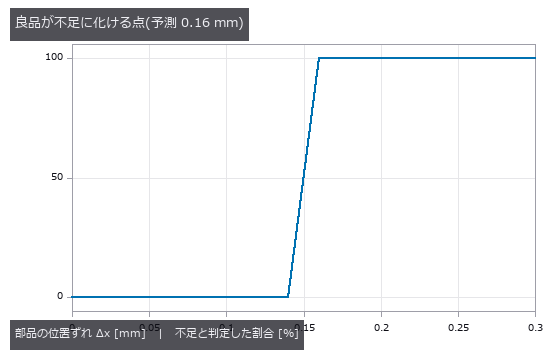
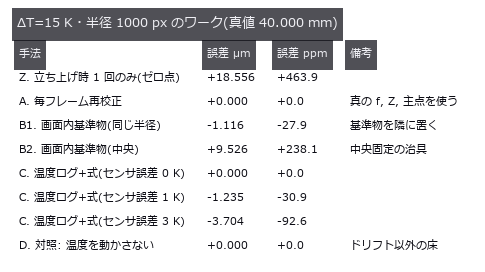
A 40 mm square measured by a camera whose focal length, mount and principal point drift with temperature ΔT, the error split into a + b·R in image radius. At ΔT = 15 K the constant term is +224.5 ppm (the single-cause control gives +225.3 ppm). Drift rises above the noise floor (23 ppm for a 25-frame average) only from ΔT = 1.6 K; below that, the honest report is that no temperature effect is visible.

↑ How Much Camera Thermal Drift Costs a Dimensional Measurement ―― A 40 mm square measured by a camera whose focal length, mount and principal point drift with temperature ΔT, the error split into a + b·R in image radius. At ΔT = 15 K the constant term is +224.5 ppm (the single-cause control gives +225.3 ppm). Drift rises above the noise floor (23 ppm for a 25-frame average) only from ΔT = 1.6 K; below that, the honest report is that no temperature effect is visible.
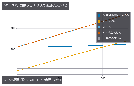
↑ The measurement ―― 焦点距離ドリフトは R に依らない。主点ドリフトは R に比例(歪みを外す中心がずれるため)。 (figure labels are in Japanese; the numbers are the same)
↑ この回の図
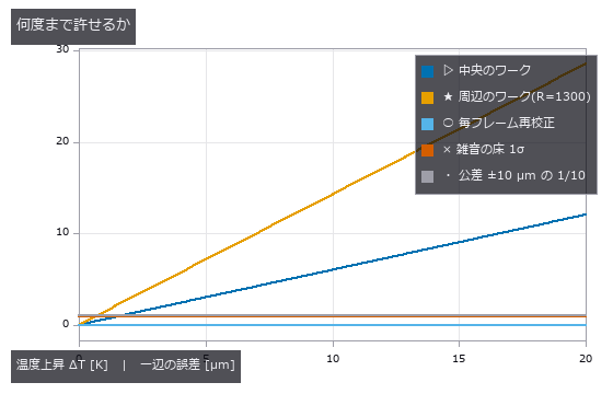
↑ 周辺のワークのほうが感度が高い。
py -3.11 examples/poc_thermal_drift_metrology.py
Source: examples/poc_thermal_drift_metrology.py
This run produced 4 figures in total - see them all
Ops used (notes): lockin_thermal_wave · polygon_area · thermo_optic_coefficient
No.2026.047 —— Veiling Glare Breaks Contrast Measurement — MTF (modulation transfer function) Passes While Black Level Fails
A PSF (point spread function) whose core stays sharp while only its tail is made heavier, with the slanted-edge MTF (modulation transfer function) and the black level of a dark square measured on the same image. Raising the tail fraction from 0 to 0.20 moves MTF50 from 0.2347 to 0.2249 cyc/px (-4.2 %, still passing) while the black level goes from 0.0 to 15.7 % (failing). A ±16 px measurement window captures only 6 % of the tail’s energy; a glare figure means nothing until the measurement extent is declared.
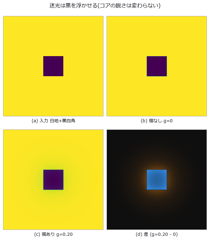
↑ Veiling Glare Breaks Contrast Measurement — MTF (modulation transfer function) Passes While Black Level Fails ―― A PSF (point spread function) whose core stays sharp while only its tail is made heavier, with the slanted-edge MTF (modulation transfer function) and the black level of a dark square measured on the same image. Raising the tail fraction from 0 to 0.20 moves MTF50 from 0.2347 to 0.2249 cyc/px (-4.2 %, still passing) while the black level goes from 0.0 to 15.7 % (failing). A ±16 px measurement window captures only 6 % of the tail’s energy; a glare figure means nothing until the measurement extent is declared.
Terms: MTF — The magnitude of the optical transfer function, showing how image contrast is transferred at each spatial frequency.; PSF — The spatial response of an imaging system to a point object, describing how that point is blurred in the image.; MTF50 — The spatial frequency at which MTF falls to 50% of its low-frequency value, used as a single-number resolution summary.
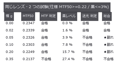
↑ The measurement (figure labels are in Japanese; the numbers are the same)
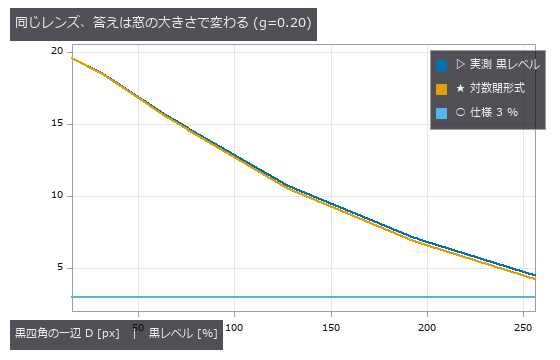
↑ D を 16 倍にすると 19.6 % が 4.5 % になる。
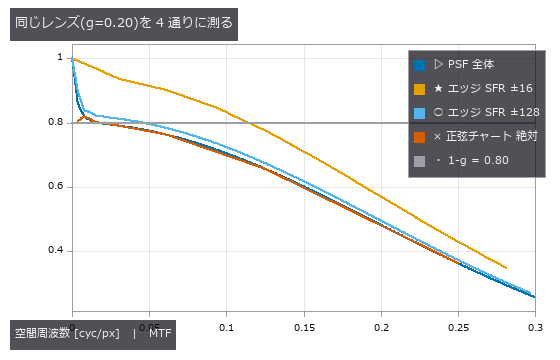
↑ 全 PSF の MTF と正弦チャートの絶対コントラストは 0.80 の台地を見る。
py -3.11 examples/poc_veiling_glare.py
Source: examples/poc_veiling_glare.py
This run produced 4 figures in total - see them all
Ops used (notes): airy_pattern · create_funct_1d_pairs · derivate_funct_1d · edge_spread · get_y_value_funct_1d · invert_funct_1d · mtf50 · mtf_diffraction · psf_to_mtf · sfr_from_edge · veiling_glare_index
No.2026.224 —— In-Camera Processing Makes Datasheet Numbers Lie Plausibly - Denoising Adds 83 % to the Quantum Efficiency, the Standard’s Check Misses It, Noise Correlation Catches It
One synthetic sensor with planted values (eta 0.45, K 0.25 DN/e-, dark noise 6 e-, 12 bit, 640 x 512, column and pixel DSNU (dark signal non-uniformity) and PRNU (photo-response non-uniformity), 30 hot pixels) is put through one in-camera processing step at a time and re-measured with the EMVA 1288 (image-sensor characterization standard) Release 4.0 Linear procedure, against the planted truth. The quantum efficiency moves by 0 % under a x2 digital gain (K +100 %, saturation capacity -51 %), by +83 % under a denoiser that mixes in 30 % of a 3 x 3 mean (0.825, still below 1 and plausible; saturation capacity +89 %, maximum SNR +2.8 dB), by -53 % under sharpening, by +87 % under recursive temporal denoising (alpha 0.8), by 0 % under factory-map defect correction (DSNU -10 %, defects 29 -> 0) and by +156 % under log companding (eta > 1, so the sensitivity-threshold operator refuses). Linear processing is predictable in closed form: with S = sum(w^2)/sum(w)^2 * alpha^2/(2 - alpha), K’ = sum(w) S K and eta’ = eta/S; prediction and measurement agree within 3 % for K, eta and sigma_d (an exact form that filters the raw quantisation noise too) and within 4 % for DSNU and PRNU with per-component gains. The standard’s equation 51 linearity check catches only the companding (171 %); denoising, sharpening and temporal filtering keep the photon transfer straight and only tilt it (0.4-1.2 %). A direct test of assumption 3 (temporal noise independent between pixels and between images; this library’s check, not a number of the standard) catches those three through the neighbour correlation of a frame difference (+0.098 / -0.072, as predicted) and the correlation with the frame after next (0.199 = 1 - alpha). Defect correction escapes every check. Release 4.0 General recovers the input SNR of the sensor behind the compander within 5 % its PRNU within 5 % and a relative quantum efficiency scan within 2 % (Linear PRNU: -39 %; equation 74 as printed is off by 589 % when the photon counts differ between wavelengths, the ratio should divide), but keeps the denoising lie: the input SNR stays 1/sqrt(S) = 1.35 times the truth, and the General SNRmax of the denoised camera reads 217, 1.71 times the truth at saturation, because saturation is set on the processed output while raw pixels clip earlier. The section 8.1 highpass drops a 9-pixel border, so one hot pixel there is invisible to section 8.8. Synthetic sensor, simplified processing, uniform illumination.

↑ In-Camera Processing Makes Datasheet Numbers Lie Plausibly - Denoising Adds 83 % to the Quantum Efficiency, the Standard’s Check Misses It, Noise Correlation Catches It ―― One synthetic sensor with planted values (eta 0.45, K 0.25 DN/e-, dark noise 6 e-, 12 bit, 640 x 512, column and pixel DSNU (dark signal non-uniformity) and PRNU (photo-response non-uniformity), 30 hot pixels) is put through one in-camera processing step at a time and re-measured with the EMVA 1288 (image-sensor characterization standard) Release 4.0 Linear procedure, against the planted truth. The quantum efficiency moves by 0 % under a x2 digital gain (K +100 %, saturation capacity -51 %), by +83 % under a denoiser that mixes in 30 % of a 3 x 3 mean (0.825, still below 1 and plausible; saturation capacity +89 %, maximum SNR +2.8 dB), by -53 % under sharpening, by +87 % under recursive temporal denoising (alpha 0.8), by 0 % under factory-map defect correction (DSNU -10 %, defects 29 -> 0) and by +156 % under log companding (eta > 1, so the sensitivity-threshold operator refuses). Linear processing is predictable in closed form: with S = sum(w^2)/sum(w)^2 * alpha^2/(2 - alpha), K’ = sum(w) S K and eta’ = eta/S; prediction and measurement agree within 3 % for K, eta and sigma_d (an exact form that filters the raw quantisation noise too) and within 4 % for DSNU and PRNU with per-component gains. The standard’s equation 51 linearity check catches only the companding (171 %); denoising, sharpening and temporal filtering keep the photon transfer straight and only tilt it (0.4-1.2 %). A direct test of assumption 3 (temporal noise independent between pixels and between images; this library’s check, not a number of the standard) catches those three through the neighbour correlation of a frame difference (+0.098 / -0.072, as predicted) and the correlation with the frame after next (0.199 = 1 - alpha). Defect correction escapes every check. Release 4.0 General recovers the input SNR of the sensor behind the compander within 5 % its PRNU within 5 % and a relative quantum efficiency scan within 2 % (Linear PRNU: -39 %; equation 74 as printed is off by 589 % when the photon counts differ between wavelengths, the ratio should divide), but keeps the denoising lie: the input SNR stays 1/sqrt(S) = 1.35 times the truth, and the General SNRmax of the denoised camera reads 217, 1.71 times the truth at saturation, because saturation is set on the processed output while raw pixels clip earlier. The section 8.1 highpass drops a 9-pixel border, so one hot pixel there is invisible to section 8.8. Synthetic sensor, simplified processing, uniform illumination.
Terms: DSNU — Spatial pixel-to-pixel variation of the mean dark signal when an image sensor receives no light.; PRNU — Spatial pixel-to-pixel variation in an image sensor’s response under uniform illumination.; EMVA 1288 — A standard measurement procedure and set of quantities for sensitivity, noise, saturation, and non-uniformity of machine-vision image sensors.

↑ The measurement ―― 拒否 = η > 1 で絶対感度しきい値(式 26)の op が拒んだ。DSNU・PRNU は照明が一様なので高域フィルタなし。 (figure labels are in Japanese; the numbers are the same)

↑ 前処理なしの差は白い砂嵐。

↑ 傾きがシステムゲイン K。

↑ General は出力の雑音を特性曲線の傾きで入力へ戻す(式 9・10)。
py -3.11 examples/poc_emva1288_in_camera_processing.py
Source: examples/poc_emva1288_in_camera_processing.py
This run produced 5 figures in total - see them all
Ops used (notes): emva_bspline_regression · emva_defect_pixels · emva_dynamic_range · emva_filter_distortion · emva_general_nonuniformity · emva_general_relative_qe · emva_general_sensitivity · emva_highpass · emva_linearity_error · emva_noise_whiteness · emva_pair_statistics · emva_photon_transfer · emva_ptc_linearity_check · emva_quantum_efficiency · emva_sensitivity_threshold · emva_snr_curve · emva_spatial_nonuniformity
No.2026.114 —— Naming the Damaged Roller from a Period — You Run Out of Evidence Before You Reach the Cliff
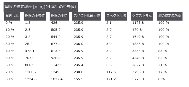
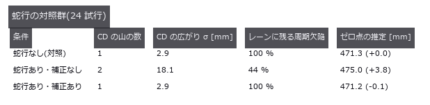
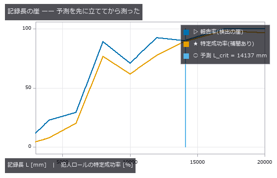
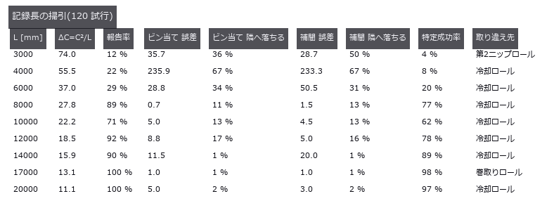
In roll-to-roll production of film, battery electrode, copper foil and paper, a single scar on a conveying roller prints itself onto the web once per roller circumference. Can the machine-direction spectrum of a defect map recover that circumference and name the culprit against a table of pi*D? Reading the naive spectral maximum names a real but innocent roller: an impulse train has a comb whose harmonics are as tall as the fundamental, so the maximum grabs C/2 = 235.62 mm, and that lands on the cooling roller at 314.16 mm in the table. A circumference that exists nowhere would be caught; one that exists elsewhere in the table passes review. That error stays at 235.9 mm as the miss rate goes from 0 to 50 % — a constant error is not evidence of robustness, it is the same mistake repeated. The fix is fail-closed: take the lowest frequency at which harmonics k=1..3 all stand. The null baseline, the median spacing between detected defects, is right when detection is perfect (-0.03 mm) but at a 40 % miss rate it errs by 472.1 mm and the mean by 813.5 mm, while the comb method holds at 3.2 mm — a missed defect removes amplitude without moving phase. A 25 mm meander, uncorrected, splits one roller’s defect line into two across the web (periodic defects remaining in the lane fall from 100 % to 44 %), yet the MD spectrum is bit-for-bit unchanged: meander only breaks methods that cut lanes in the cross direction. Sixty control trials with only healthy rollers give a 1.7 % false-positive rate, and the floor is not zero — the healthy side reaches 3.99 times the band median, above the 2.5 threshold on its own, so what actually holds the line is the demand that every harmonic stand. There are two cliffs. The prediction L_crit = C^2/dC = 14137 mm matches the measured resolution cliff at 14000 mm, a ratio of 0.99. But the detection cliff, the shortest record that still always reports, is 17000 mm — longer. Shortening the record makes you say nothing before it makes you say the wrong roller, so the cliff Rayleigh predicted correctly is never reached. The criterion itself needed repair: at 24 trials a clean 0 % existed, at 120 trials 2 % survives even at the longest record, so 0 % was a small-sample artefact rather than a floor. The most frequent wrong answer, at seven of nine sweep points, is the cooling roller, and 471.24 / 314.16 = 1.500 is exactly 3:2: an integer ratio inside the table gives the comb method a misidentification of its own. The two gaps this PoC found have since been filled: fs.point_spectrum takes a periodogram straight from event positions and carries its own resolution in the return value, and fs.peak_subbin refines a peak below the bin without clamping the shift, since a vertex further than half a sample away means the index was not a maximum at all.
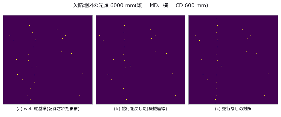
↑ Naming the Damaged Roller from a Period — You Run Out of Evidence Before You Reach the Cliff ―― In roll-to-roll production of film, battery electrode, copper foil and paper, a single scar on a conveying roller prints itself onto the web once per roller circumference. Can the machine-direction spectrum of a defect map recover that circumference and name the culprit against a table of piD? Reading the naive spectral maximum names a real but innocent roller: an impulse train has a comb whose harmonics are as tall as the fundamental, so the maximum grabs C/2 = 235.62 mm, and that lands on the cooling roller at 314.16 mm in the table. A circumference that exists nowhere would be caught; one that exists elsewhere in the table passes review. That error stays at 235.9 mm as the miss rate goes from 0 to 50 % — a constant error is not evidence of robustness, it is the same mistake repeated. The fix is fail-closed: take the lowest frequency at which harmonics k=1..3 all stand. The null baseline, the median spacing between detected defects, is right when detection is perfect (-0.03 mm) but at a 40 % miss rate it errs by 472.1 mm and the mean by 813.5 mm, while the comb method holds at 3.2 mm — a missed defect removes amplitude without moving phase. A 25 mm meander, uncorrected, splits one roller’s defect line into two across the web (periodic defects remaining in the lane fall from 100 % to 44 %), yet the MD spectrum is bit-for-bit unchanged: meander only breaks methods that cut lanes in the cross direction. Sixty control trials with only healthy rollers give a 1.7 % false-positive rate, and the floor is not zero — the healthy side reaches 3.99 times the band median, above the 2.5 threshold on its own, so what actually holds the line is the demand that every harmonic stand. There are two cliffs. The prediction L_crit = C^2/dC = 14137 mm matches the measured resolution cliff at 14000 mm, a ratio of 0.99. But the detection cliff, the shortest record that still always reports, is 17000 mm — longer. Shortening the record makes you say nothing before it makes you say the wrong roller, so the cliff Rayleigh predicted correctly is never reached. The criterion itself needed repair: at 24 trials a clean 0 % existed, at 120 trials 2 % survives even at the longest record, so 0 % was a small-sample artefact rather than a floor. The most frequent wrong answer, at seven of nine sweep points, is the cooling roller, and 471.24 / 314.16 = 1.500 is exactly 3:2: an integer ratio inside the table gives the comb method a misidentification of its own. The two gaps this PoC found have since been filled: fs.point_spectrum takes a periodogram straight from event positions and carries its own resolution in the return value, and fs.peak_subbin refines a peak below the bin without clamping the shift, since a vertex further than half a sample away means the index was not a maximum at all.*

↑ The measurement ―― 見逃しは位相を飛ばさないので、櫛の山は低くなるだけで動かない。 (figure labels are in Japanese; the numbers are the same)
↑ この回の図
↑ この回の図
↑ 縦線が閉形式の予測 C²/ΔC。
↑ この回の図
py -3.11 examples/poc_web_roll_periodicity.py
Source: examples/poc_web_roll_periodicity.py
This run produced 10 figures in total - see them all
Ops used (notes): cepstrum · find_peaks · local_min_max_funct_1d · median · peak_subbin · point_spectrum · smooth_funct_1d_gauss · spectrum
No.2026.050 —— Weld Bead From a Laser-Triangulation Profile — The Sin of Writing 0 Where Nothing Was Measured
The profile h(x) recovered from the row position of a single laser line, with reinforcement height, width and undercut read off it. The centroid beats the null (integer argmax per column) by 9.3x, and with zero noise the log-parabola is exact to machine precision, 12 orders better than a plain parabola; at 1 % noise the two are 0.00272 versus 0.00260 mm, indistinguishable. Five spatter points break all three estimators together to 0.11 mm (40x); what matters is not refinement but which peak you pick.
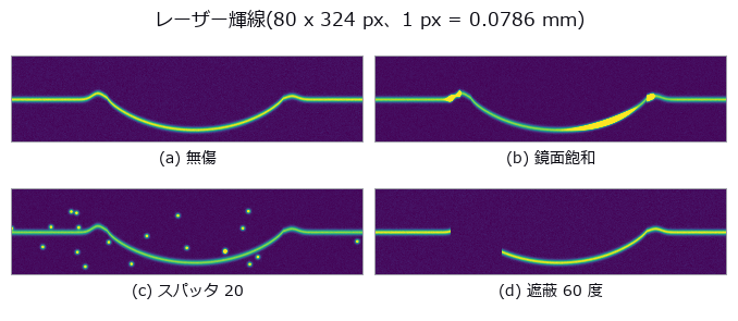
↑ Weld Bead From a Laser-Triangulation Profile — The Sin of Writing 0 Where Nothing Was Measured ―― The profile h(x) recovered from the row position of a single laser line, with reinforcement height, width and undercut read off it. The centroid beats the null (integer argmax per column) by 9.3x, and with zero noise the log-parabola is exact to machine precision, 12 orders better than a plain parabola; at 1 % noise the two are 0.00272 versus 0.00260 mm, indistinguishable. Five spatter points break all three estimators together to 0.11 mm (40x); what matters is not refinement but which peak you pick.
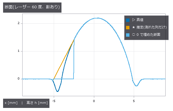
↑ The measurement ―― 0 で埋めた線は影の区間で h=0 に張り付き、左のアンダーカットが消えて偽のつま先ができる。 (figure labels are in Japanese; the numbers are the same)

↑ 真値 0.45 mm。
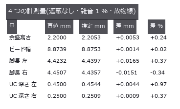
↑ 遮蔽が無ければ全部 1 % 以内。
py -3.11 examples/poc_weld_bead_profile.py
Source: examples/poc_weld_bead_profile.py
This run produced 4 figures in total - see them all
Ops used (notes): gen_measure_rectangle2 · measure_pos · median · smooth_funct_1d_mean
No.2026.115 —— Light-section scanning of a weld bead — resolution and occlusion share one knob
A fillet-weld cross-section is built in closed form with convexity, leg lengths, throat and undercut depth varied along the weld line by known functions, then the triangulation angle is swept from 15 to 70 degrees. Height resolution improves as 1/sin(theta) while any face rising steeper than cot(theta) hides in its own shadow, so the far parent plate turns away exactly at the predicted 37.0 degrees and the far undercut starts vanishing earlier, at 20.8-34.5 degrees (the deeper the groove, the sooner). The dangerous parts are that at 28 degrees every cross-section still reports a value while 25 % of the groove span is unmeasured and the depth reads 27 % shallow, and that raising the angle further drops the deepest cross-sections out of the average (true mean drifting 0.260 to 0.047 mm) — a survivorship bias; the optimal angle differs per measurand at 20 / 24 / 36 / 64 degrees.
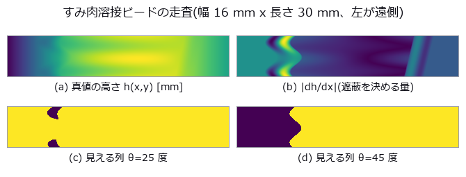
↑ Light-section scanning of a weld bead — resolution and occlusion share one knob ―― A fillet-weld cross-section is built in closed form with convexity, leg lengths, throat and undercut depth varied along the weld line by known functions, then the triangulation angle is swept from 15 to 70 degrees. Height resolution improves as 1/sin(theta) while any face rising steeper than cot(theta) hides in its own shadow, so the far parent plate turns away exactly at the predicted 37.0 degrees and the far undercut starts vanishing earlier, at 20.8-34.5 degrees (the deeper the groove, the sooner). The dangerous parts are that at 28 degrees every cross-section still reports a value while 25 % of the groove span is unmeasured and the depth reads 27 % shallow, and that raising the angle further drops the deepest cross-sections out of the average (true mean drifting 0.260 to 0.047 mm) — a survivorship bias; the optimal angle differs per measurand at 20 / 24 / 36 / 64 degrees.
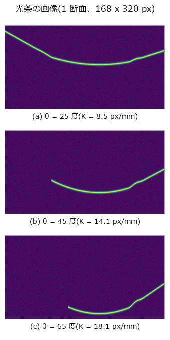
↑ The measurement ―― θ を大きくすると高さの伸び K が増えて分解能は上がる(輝線の起伏が大きくなる)が、左半分の輝線が消えていく。 (figure labels are in Japanese; the numbers are the same)

↑ θ = 28 度。

↑ 下に凸の谷がアンダーカット。

↑ 同じノブの表裏。
↑ 脚長は sin²(母材角)、溝深さは cos²(母材角) —— 同じ母材面で足すと 1。
py -3.11 examples/poc_weld_bead_scan_angle.py
Source: examples/poc_weld_bead_scan_angle.py
This run produced 11 figures in total - see them all
Ops used (notes): esdf · fit_plane_3d · intersect_planes · lines_gauss · normals_from_depth · occupancy_grid · query_distance
No.2026.122 —— Finding and Fixing Wrong Characters Without Recognising Them — the Threshold Comes from Typeface Spread
Because the intended string is given as input, no 6000-way classification is needed: each cell is compared against one specified character. The threshold is not guessed but derived from the 95th percentile of the distance between the same character in different typefaces (0.058). The distance is the 99th percentile rather than the mean — a substitution usually keeps one radical and swaps the rest, so the mean sinks the 検/横 pair to 0.0171, below the typeface floor, making it undetectable in principle. On a synthetic sign all four planted errors are found with no false alarms, and after replacement the distance drops from 0.0805 to 0.0325, below the floor for all four.

↑ Finding and Fixing Wrong Characters Without Recognising Them — the Threshold Comes from Typeface Spread ―― Because the intended string is given as input, no 6000-way classification is needed: each cell is compared against one specified character. The threshold is not guessed but derived from the 95th percentile of the distance between the same character in different typefaces (0.058). The distance is the 99th percentile rather than the mean — a substitution usually keeps one radical and swaps the rest, so the mean sinks the 検/横 pair to 0.0171, below the typeface floor, making it undetectable in principle. On a synthetic sign all four planted errors are found with no false alarms, and after replacement the distance drops from 0.0805 to 0.0325, below the floor for all four.

↑ The measurement ―― 床を超えたマスが誤字。壊した位置は 2, 3, 5, 7。 (figure labels are in Japanese; the numbers are the same)
py -3.11 examples/poc_glyph_typo_detection.py
Source: examples/poc_glyph_typo_detection.py
This run produced 2 figures in total - see them all
No.2026.130 —— Print Layer Inspection — Closing the Shape → Layer → Path → Image Loop and Catching Planted Defects by the Numbers
3D-printer data flows shape (mesh) → layers (slices) → path (G-code) → the layer images taken during printing. The new family printpath (11 ops, numpy + stdlib, no new types) closes that loop with the existing vocabulary (mesh / voxel / table / image2d), so the truth can be planted by hand. A box with a square hole and a gear-like boss with a round hole sliced at 0.2 mm give layer-mask areas matching the closed form (184.00 mm² exactly and within 0.07 %), a layer where only the hole remains is empty (contours oriented by the triangle normals, nonzero winding), the extrusion of a path that walks the contours equals perimeter × width × height / filament area exactly, G-code round-trips through write and read (relative coordinates, relative E, retracts, G92 and inches are honoured; arcs and missing coordinates are refused), and 3MF round-trips too. Inspection: six gaps and six blobs (1–4 mm) planted into the expected layer raster (gcode_layer_image) are caught by print_layer_defect_map with sign, recall 0.959 and zero false positives at a 3 px (0.3 mm) tolerance; a 0.2 mm camera shift drops recall to 0.895 and precision to 0.946 because the tolerance eats the defect edges — the curve over tolerance is shown as it is.
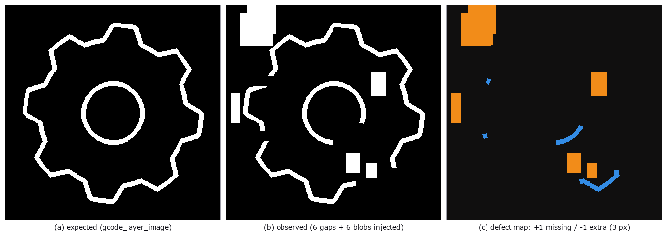
↑ Print Layer Inspection — Closing the Shape → Layer → Path → Image Loop and Catching Planted Defects by the Numbers ―― 3D-printer data flows shape (mesh) → layers (slices) → path (G-code) → the layer images taken during printing. The new family printpath (11 ops, numpy + stdlib, no new types) closes that loop with the existing vocabulary (mesh / voxel / table / image2d), so the truth can be planted by hand. A box with a square hole and a gear-like boss with a round hole sliced at 0.2 mm give layer-mask areas matching the closed form (184.00 mm² exactly and within 0.07 %), a layer where only the hole remains is empty (contours oriented by the triangle normals, nonzero winding), the extrusion of a path that walks the contours equals perimeter × width × height / filament area exactly, G-code round-trips through write and read (relative coordinates, relative E, retracts, G92 and inches are honoured; arcs and missing coordinates are refused), and 3MF round-trips too. Inspection: six gaps and six blobs (1–4 mm) planted into the expected layer raster (gcode_layer_image) are caught by print_layer_defect_map with sign, recall 0.959 and zero false positives at a 3 px (0.3 mm) tolerance; a 0.2 mm camera shift drops recall to 0.895 and precision to 0.946 because the tolerance eats the defect edges — the curve over tolerance is shown as it is.
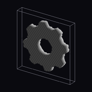
↑ The measurement ―― gear-like boss with a round hole sliced at 0.2 mm into 30 layer masks (mesh_slice_stack) and rendered as a solid, grey = height (figure labels are in Japanese; the numbers are the same)
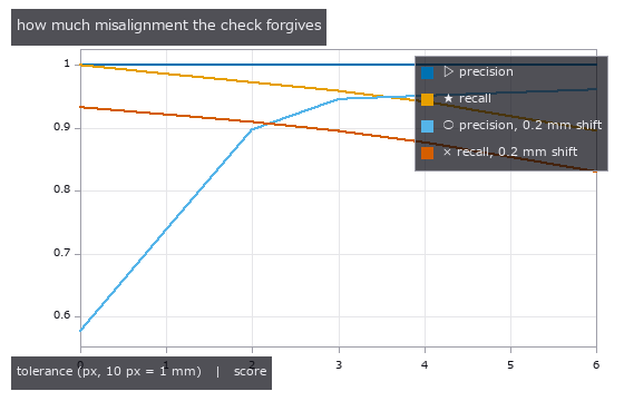
↑ precision and recall of the defect map against the injected truth as the tolerance grows, without and with a 0.2 mm camera shift: a small tolerance ab…
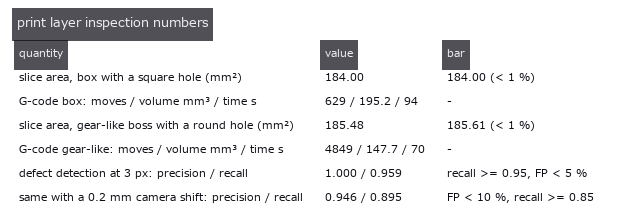
↑ every number with the bar it had to clear
py -3.11 examples/poc_print_layer_inspection.py
Source: examples/poc_print_layer_inspection.py
This run produced 4 figures in total - see them all
Ops used (notes): contours_to_gcode · gcode_extrusion_volume · gcode_layer_image · gcode_read · gcode_time_estimate · gcode_write · mesh_slice_contours · mesh_slice_stack · print_layer_defect_map · prism_mesh · read_3mf · vol_render_transfer · write_3mf
No.2026.189 —— A Warehouse That Does Not Jam When Vehicles Run Late — A Correct Plan Alone Still Stops an AGV Fleet
The author’s remark: “we have done nothing on AGVs, the simple vehicles manufacturing uses everywhere”. A transport plan for 12 vehicles on a floor grid is built with focal-search CBS (cost 96 ≤ 1.1 × lower bound 88), then executed 1000 times with each vehicle delayed with probability 0.3 per step. Naive execution (“move if the next cell is free”) jams in 641 of 1000 runs; execution that follows the action dependency graph (ADG, Hönig et al. 2019) has 0 collisions and 0 deadlocks. Of the 641 jams, 640 were a vehicle that had arrived and stayed parked in the aisle; only 1 was a cycle of waits. Gates: the CBS sum of costs matches the optimum of A* over the joint state of all vehicles (a second implementation) in 40 / 40 cases, focal search ≤ 1.3 × optimum in 40 / 40, a concrete instance that prioritized planning cannot solve in any order (CBS and joint A* both cost 9), and every VDA 5050 order passes the structural rules. Honestly: one step is a fixed time on a discrete grid; acceleration, turning and vehicle size are not modelled.
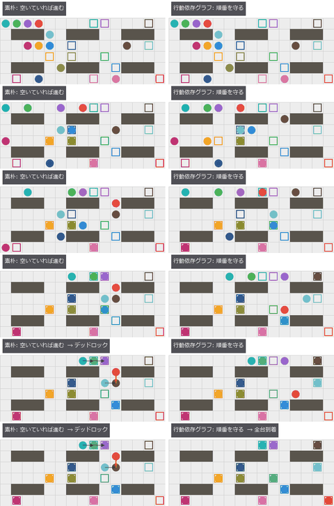
↑ A Warehouse That Does Not Jam When Vehicles Run Late — A Correct Plan Alone Still Stops an AGV Fleet ―― The author’s remark: “we have done nothing on AGVs, the simple vehicles manufacturing uses everywhere”. A transport plan for 12 vehicles on a floor grid is built with focal-search CBS (cost 96 ≤ 1.1 × lower bound 88), then executed 1000 times with each vehicle delayed with probability 0.3 per step. Naive execution (“move if the next cell is free”) jams in 641 of 1000 runs; execution that follows the action dependency graph (ADG, Hönig et al. 2019) has 0 collisions and 0 deadlocks. Of the 641 jams, 640 were a vehicle that had arrived and stayed parked in the aisle; only 1 was a cycle of waits. Gates: the CBS sum of costs matches the optimum of A over the joint state of all vehicles (a second implementation) in 40 / 40 cases, focal search ≤ 1.3 × optimum in 40 / 40, a concrete instance that prioritized planning cannot solve in any order (CBS and joint A* both cost 9), and every VDA 5050 order passes the structural rules. Honestly: one step is a fixed time on a discrete grid; acceleration, turning and vehicle size are not modelled.*

↑ The measurement ―― 最後のコマ(左: デッドロック、右: 全台到着) (figure labels are in Japanese; the numbers are the same)

↑ 同じ 12 台の計画を、遅れの確率ごとに 200 通り走らせたデッドロックの割合。
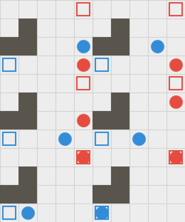
↑ The animation ―― 優先度付き計画が、どちらを先にしても解けない問題(CBS の総コスト 9)。CBS は片方に道を譲らせて解く
py -3.11 examples/poc_agv_fleet.py
Source: examples/poc_agv_fleet.py
This run produced 4 figures in total - see them all
Ops used (notes): adg_build · adg_execute · arrow · mapf_cbs · mapf_ecbs · mapf_joint_astar · mapf_prioritized · naive_execute · plan_conflicts · text_box · vda5050_check · vda5050_order · warehouse_grid
No.2026.223 —— Find Hybrid-Bond Voids by Echo Phase, Not Brightness - Small Voids Hide in the Amplitude Image and Light Up Inverted in the Phase Image
A thinned 100 um silicon die over a hybrid bond (SiO2 1 + 1 um, Cu pads 1 + 1 um of 40 um diameter at 80 um pitch) with voids of 5 to 24 um placed on pads and in the dielectric, imaged by a focused scanning acoustic microscope (1 mm of water, F/3); echoes come from a layer transfer matrix checked against a bottom-up Airy recursion (Airy multiple-reflection formula), a time-domain ray sum and the optical thin-film formula to 1e-12. Read at the expected time of the bond plane, the dielectric echo is at -91 deg and the Cu pad at +84 deg (thin layers give quadrature echoes) while voids are inverted (-175 deg in the dielectric, +159 deg on a pad). In the amplitude image 8 of 12 voids hide inside the brightness range of intact pixels: an inverted echo adds at right angles to a quadrature background, so voids of 9 to 16 um change the amplitude by 0.4 to 3.5 sigma but the phase-aware statistic by 3.0 to 8.9 sigma; the phase image flags every void of 16 um and up and 1 of 26,724 intact pixels. The conventional single-sample polarity of an intact Cu pad flips 5 times between 140 and 400 MHz. The optimal frequency has a closed form (139.16 MHz for a 10 um void, equal to brute force) and the front-echo tail sets a floor of 130 MHz. POD (a-hat vs a, 88 voids): a90/95 of the phase-aware detector is 12.4 / 13.9 / 57.6 um at 150 / 200 / 300 MHz against 16.6 / 19.3 / 101.6 um for amplitude only, under the same baseline and threshold rule. Synthetic: 1-D plane-wave longitudinal layers, a Gaussian lateral PSF, no refraction aberration, silicon attenuation set to 0 (unverified), no kissing bonds.

↑ Find Hybrid-Bond Voids by Echo Phase, Not Brightness - Small Voids Hide in the Amplitude Image and Light Up Inverted in the Phase Image ―― A thinned 100 um silicon die over a hybrid bond (SiO2 1 + 1 um, Cu pads 1 + 1 um of 40 um diameter at 80 um pitch) with voids of 5 to 24 um placed on pads and in the dielectric, imaged by a focused scanning acoustic microscope (1 mm of water, F/3); echoes come from a layer transfer matrix checked against a bottom-up Airy recursion (Airy multiple-reflection formula), a time-domain ray sum and the optical thin-film formula to 1e-12. Read at the expected time of the bond plane, the dielectric echo is at -91 deg and the Cu pad at +84 deg (thin layers give quadrature echoes) while voids are inverted (-175 deg in the dielectric, +159 deg on a pad). In the amplitude image 8 of 12 voids hide inside the brightness range of intact pixels: an inverted echo adds at right angles to a quadrature background, so voids of 9 to 16 um change the amplitude by 0.4 to 3.5 sigma but the phase-aware statistic by 3.0 to 8.9 sigma; the phase image flags every void of 16 um and up and 1 of 26,724 intact pixels. The conventional single-sample polarity of an intact Cu pad flips 5 times between 140 and 400 MHz. The optimal frequency has a closed form (139.16 MHz for a 10 um void, equal to brute force) and the front-echo tail sets a floor of 130 MHz. POD (a-hat vs a, 88 voids): a90/95 of the phase-aware detector is 12.4 / 13.9 / 57.6 um at 150 / 200 / 300 MHz against 16.6 / 19.3 / 101.6 um for amplitude only, under the same baseline and threshold rule. Synthetic: 1-D plane-wave longitudinal layers, a Gaussian lateral PSF, no refraction aberration, silicon attenuation set to 0 (unverified), no kissing bonds.
Terms: SAM — An instrument that scans focused ultrasound over a specimen and images internal interfaces or defects from echo amplitude, phase, or arrival time.; Airy — The formula for a parallel plate’s transmittance obtained by summing its infinite series of multiple reflections.
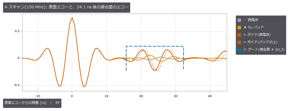
↑ The measurement ―― 接合面のエコーは表面エコーの 1 割未満。ボイドのエコーは反転、誘電体とパッドは直交(微分形)。 (figure labels are in Japanese; the numbers are the same)

↑ 期待時刻(24.1 ns)で読んだ位相は、誘電体 -91°、Cu パッド +84°、ボイド(誘電体) -175°、ボイド(パッドの上) +159°。
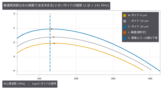
↑ S(f) = (1 − 2^−(a/w)²) exp(−β f²)。

↑ FWHM = 1.02 λ_w F#(F# 3)、水の経路 1 mm(2.17e-3 dB/(cm MHz²))。
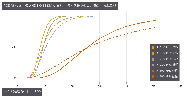
↑ 閾値は同じ規則(良品の部位の平均 + 3.09σ、パッドと誘電体の厳しい方)。
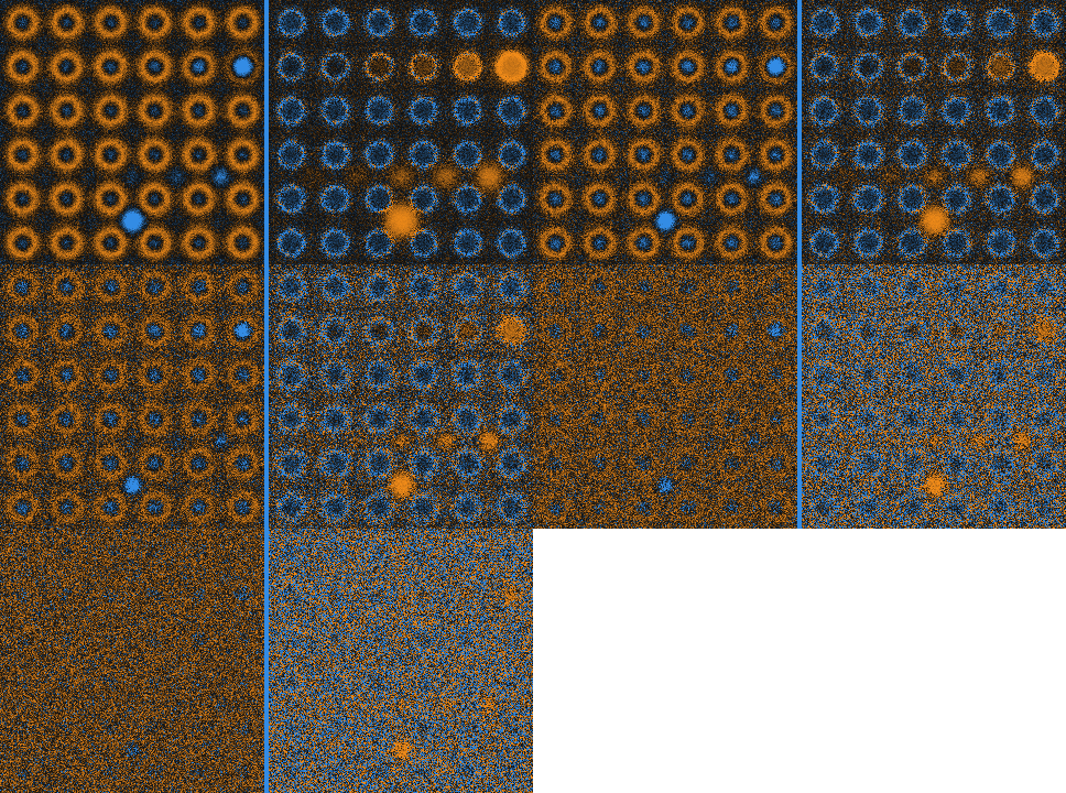
↑ The animation ―― 150 → 350 MHz。左 = 振幅(各コマで正規化)、右 = cos(位相)。周波数を上げると像は締まるが、水の減衰で雑音に沈んでいく。
py -3.11 examples/poc_sam_hybrid_bonding_voids.py
Source: examples/poc_sam_hybrid_bonding_voids.py
This run produced 8 figures in total - see them all
Ops used (notes): acoustic_interface_coefficients · acoustic_material_table · echo_phase_polarity · pod_ahat_fit · pod_false_call · pod_from_ahat · pulse_echo_ascan · sam_cscan · sam_frequency_tradeoff
No.2026.226 —— Why a Thin Groove Vanishes in a PL Image — a Longer Diffusion Length Hides Only Shadow Grooves, and Makes Sink Grooves Stand Out
A photoluminescence (PL) image glows only after the excess carriers have diffused, so a second PSF (point spread function) set by the diffusion length L = sqrt(D tau) (the 2-D Green function K0(r/L)/2 pi L^2) sits on top of the optical one. Three new ops: pl_diffusion_psf (the kernel, sum 1), pl_image_simulate (an exact grid solve of the steady-state diffusion equation from an excitation map and a recombination map) and pl_groove_visibility (closed-form contrast, CNR and visibility boundary L* from groove width, diffusion length and noise). The pre-run prediction that the same groove fades on a better wafer with a longer diffusion length came out half right: a shadow groove (missing excitation, 1 - exp(-w/2L)) fades from 11.8 to 1.6 % as L goes 20 to 160 um, but a sink groove (a recombination line, Donolato’s SL/(SL+2D)) deepens from 48.9 to 89.0 % (grid closed form to 1e-10, continuous form within 2.4 %, Donolato within 1.7 %). Public measured data (laser grooves in Si wafers after HF treatment at 0 min / 55 min / 1 week, CC BY 4.0, DOI 10.5281/zenodo.19603335) are read from the raw images, the paper’s histogram (L1 0) and line scans (RMS within 1.1 %) are reproduced first, and then the groove is deeper (50 to 35 %) and wider (FWHM 1.32 to 0.42 mm) right after HF: the sink direction. The PL level is no proxy for the diffusion length (55 min has the lowest level but intermediate depth and width). In an embedded-groove POD the longer-L 0 min ground makes the shadow a90 4.6 times larger (hidden) and the sink a90 0.28 times (revealed); the measured a90 is more than an order of magnitude looser than the white-noise closed form, so the limit is set by the structure of the ground, not by noise. The real-data stage runs only when the environment variable is set; no data is bundled.

↑ Why a Thin Groove Vanishes in a PL Image — a Longer Diffusion Length Hides Only Shadow Grooves, and Makes Sink Grooves Stand Out ―― A photoluminescence (PL) image glows only after the excess carriers have diffused, so a second PSF (point spread function) set by the diffusion length L = sqrt(D tau) (the 2-D Green function K0(r/L)/2 pi L^2) sits on top of the optical one. Three new ops: pl_diffusion_psf (the kernel, sum 1), pl_image_simulate (an exact grid solve of the steady-state diffusion equation from an excitation map and a recombination map) and pl_groove_visibility (closed-form contrast, CNR and visibility boundary L from groove width, diffusion length and noise). The pre-run prediction that the same groove fades on a better wafer with a longer diffusion length came out half right: a shadow groove (missing excitation, 1 - exp(-w/2L)) fades from 11.8 to 1.6 % as L goes 20 to 160 um, but a sink groove (a recombination line, Donolato’s SL/(SL+2D)) deepens from 48.9 to 89.0 % (grid closed form to 1e-10, continuous form within 2.4 %, Donolato within 1.7 %). Public measured data (laser grooves in Si wafers after HF treatment at 0 min / 55 min / 1 week, CC BY 4.0, DOI 10.5281/zenodo.19603335) are read from the raw images, the paper’s histogram (L1 0) and line scans (RMS within 1.1 %) are reproduced first, and then the groove is deeper (50 to 35 %) and wider (FWHM 1.32 to 0.42 mm) right after HF: the sink direction. The PL level is no proxy for the diffusion length (55 min has the lowest level but intermediate depth and width). In an embedded-groove POD the longer-L 0 min ground makes the shadow a90 4.6 times larger (hidden) and the sink a90 0.28 times (revealed); the measured a90 is more than an order of magnitude looser than the white-noise closed form, so the limit is set by the structure of the ground, not by noise. The real-data stage runs only when the environment variable is set; no data is bundled.*
Terms: PSF — The spatial response of an imaging system to a point object, describing how that point is blurred in the image.

↑ The measurement ―― 同じ幅 3 µm の溝を拡散長 L = 4 / 16 / 64 µm で描いた PL 像(雑音 1 %)。上段 = 影の溝(励起の欠け): L が長いほど拡散が埋めて消える。下段 = 沈みの溝(再結合の線): L が長いほど深く・広く見える。良質なウェハで隠れるのは影だけ。 (figure labels are in Japanese; the numbers are the same)

↑ 幅 5 µm の溝の中心コントラスト対拡散長(閉形式)。
py -3.11 examples/poc_si_wafer_pl_defect_visibility.py
Source: examples/poc_si_wafer_pl_defect_visibility.py
This run produced 3 figures in total - see them all
Ops used (notes): pl_diffusion_psf · pl_groove_visibility · pl_image_simulate · pod_hitmiss_fit
No.2026.240 —— Illumination Cone versus Imaging NA — Change Only the Opening of the Light Cone and the Same Dent, Scratch and Satin Patch Vanish or Appear
| For shallow dents, scratches on a hairline finish and satin unevenness on near-specular metal parts, what shows is set less by the type of light than by the half-angle α and axis of the cone of light reaching each point, relative to the cone the camera accepts (object-side NA, half-angle β): the illumination-NA / objective-NA relation of Koehler illumination and the knife edge of schlieren optics. Reflection is an isometry of the sphere of directions, so the brightness is the intersection of two spherical caps, a closed form: slopes below | α − β | /2 do not show, slopes beyond (α + β)/2 go dark. Five new ops in illumdesign (solid_angle_light, solid_angle_boundaries, solid_angle_brightness, solid_angle_sweep, solid_angle_render). The closed form agrees with the projected-solid-angle pupil integral to 0.002. Through a telecentric lens of NA 0.033 a 2 µm dent (steepest slope 0.25°) shows as a ring only with α = β (contrast −0.091 measured on the image, closed form to 1e-4) and vanishes at α = 0.5° and 7°, as the closed form predicts. The closed form picks α between 3.5° and 6.1° to hide hairline marks (99th-percentile slope 0.82°) while blackening a 4° scratch: at α = 4° the marks fluctuate 0.014 times as much as at α = β and the scratch contrast is −1.00. Tilting the cone by β puts the flat ground at 0.39 and splits the dent’s flanks into 0.53 and 0.25 (closed form 0.54 / 0.25), so the slope sign reads as bright or dark. Satin patches (micro-facet spread 1.3° against 0.8°) give −0.20 at α = β and −0.02 at α = 7°. Where it breaks: ±0.25° waviness makes the background swing 1.6 times the dent’s dip at α = β, so a threshold cannot pick the dent; a micro-facet spread of 0.25° already cuts the contrast to a third, and at 4° no cone gets above 0.001. No comparison photographs taken with only the illumination solid angle changed were found under a reusable licence, so the check against real images is still open. Nothing learned, nothing calibrated, 15 gates. |

| *↑ Illumination Cone versus Imaging NA — Change Only the Opening of the Light Cone and the Same Dent, Scratch and Satin Patch Vanish or Appear ―― For shallow dents, scratches on a hairline finish and satin unevenness on near-specular metal parts, what shows is set less by the type of light than by the half-angle α and axis of the cone of light reaching each point, relative to the cone the camera accepts (object-side NA, half-angle β): the illumination-NA / objective-NA relation of Koehler illumination and the knife edge of schlieren optics. Reflection is an isometry of the sphere of directions, so the brightness is the intersection of two spherical caps, a closed form: slopes below | α − β | /2 do not show, slopes beyond (α + β)/2 go dark. Five new ops in illumdesign (solid_angle_light, solid_angle_boundaries, solid_angle_brightness, solid_angle_sweep, solid_angle_render). The closed form agrees with the projected-solid-angle pupil integral to 0.002. Through a telecentric lens of NA 0.033 a 2 µm dent (steepest slope 0.25°) shows as a ring only with α = β (contrast −0.091 measured on the image, closed form to 1e-4) and vanishes at α = 0.5° and 7°, as the closed form predicts. The closed form picks α between 3.5° and 6.1° to hide hairline marks (99th-percentile slope 0.82°) while blackening a 4° scratch: at α = 4° the marks fluctuate 0.014 times as much as at α = β and the scratch contrast is −1.00. Tilting the cone by β puts the flat ground at 0.39 and splits the dent’s flanks into 0.53 and 0.25 (closed form 0.54 / 0.25), so the slope sign reads as bright or dark. Satin patches (micro-facet spread 1.3° against 0.8°) give −0.20 at α = β and −0.02 at α = 7°. Where it breaks: ±0.25° waviness makes the background swing 1.6 times the dent’s dip at α = β, so a threshold cannot pick the dent; a micro-facet spread of 0.25° already cuts the contrast to a third, and at 4° no cone gets above 0.001. No comparison photographs taken with only the illumination solid angle changed were found under a reusable licence, so the check against real images is still open. Nothing learned, nothing calibrated, 15 gates.* |
| [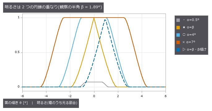](https://raw.githubusercontent.com/furuse-kazufumi/fullseye/master/docs/articles/assets/poc/poc_illumination_cone_vs_na/01_brightness_vs_slope.png) |
| *↑ The measurement ―― 鏡面の傾き θ と、カメラの瞳が反射した光の円錐で覆われる割合(閉形式)。α = 7° と 0.5° は傾き | α − β | /2 まで平らで、そこまでの傾きは見えない。α = β は 0 から下がり始めるので最も小さな傾きが見える。β だけ傾けた円錐は平らな地が半分の明るさで、傾きの向きで明るくも暗くもなる。 (figure labels are in Japanese; the numbers are the same)* |

↑ 傾き θ の面と平らな地のコントラストを α に対して(微小面の粗さ 0)。

↑ 面のうねり(周期 1.5 mm、傾き ±0.25°)を足した鏡面の打痕。

↑ α を 0.5〜3° から選んだ最大のコントラスト。
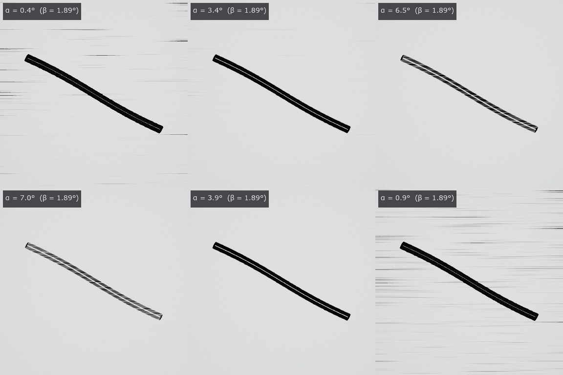
↑ The animation ―― ヘアラインの上の傷を、照明の円錐の半角 α だけを 0.4〜8° で往復させて撮る。α ≈ β で筋が最も目立ち、α ≈ 4° で筋が消えて傷が黒く残り、広げすぎると傷も薄れる。
py -3.11 examples/poc_illumination_cone_vs_na.py
Source: examples/poc_illumination_cone_vs_na.py
This run produced 6 figures in total - see them all
Ops used (notes): blast_normals · light_source · metal_mirror_rgb · micro_normals · solid_angle_boundaries · solid_angle_brightness · solid_angle_light · solid_angle_render · solid_angle_sweep · text_box
No.2026.254 —— Matching on the Direction of Brightness Change — NCC Falls at 10 % Occlusion, Code Matching Holds to Over 60 %
Normalised cross-correlation, the usual template matcher, fails when part of the target is hidden or glare washes it out. Matchers comparing the sign of brightness changes were tested on 40 templates from public real photos. They withstand occlusion far better, yet every method stays weak to rotation.
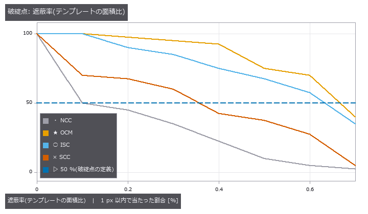
| *↑ Matching on the Direction of Brightness Change — NCC Falls at 10 % Occlusion, Code Matching Holds to Over 60 % ―― Normalised cross-correlation (NCC) compares brightness values, so it is fragile when part of the template is occluded, saturated by a highlight or darkened on one side. Four matchers that compare the direction of brightness change as codes (orientation code matching, increment sign correlation, the selective correlation coefficient and the Radial Reach Filter, re-implemented from the published equations) are added as six codematch ops and scored on 40 templates of 32 x 32 cut from five public CC0 photographs. Half the hits are lost at 10 % occlusion for NCC, 36 % for SCC, 63 % for ISC and 67 % for OCM; at 6 %, 10 %, 44 % and 53 % saturated highlight. All four are weak to rotation (7-9 degrees). SCC selects only pixels whose codes agree, which inflates correlation at unrelated positions (selection bias); taken literally it broke before NCC, and a floor at the uncorrelated usage rate plus 4 sigma fixes it. On 11 flat sky templates NCC misses 10 with correlation around 0.82, while the code matchers refuse or answer correctly (no wrong answer). Gates: a brute-force second implementation, the existing NCC, invariance to monotone maps, commutation with rot90 (broken by a probe that swaps the cyclic difference for the absolute one) and a closed-form model of the values at the true position ( | z | <= 3.6 over 1,080 trials).* |
Terms: OCM — A template-matching method that quantizes each pixel’s gradient orientation and compares the resulting orientation codes.
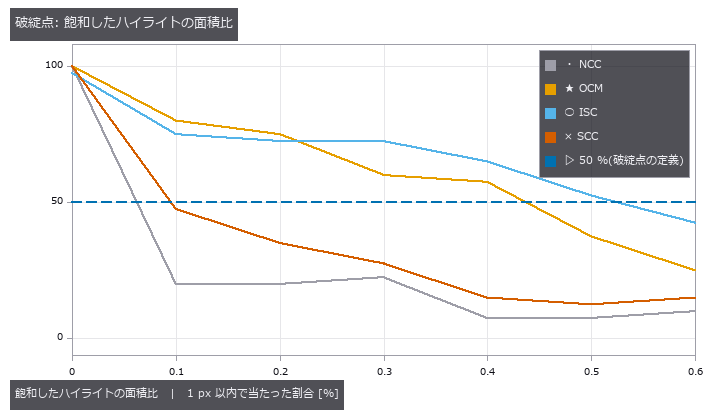
↑ The measurement ―― 公開の実写 5 枚から切った 32 x 32 のテンプレートを、雑音 σ = 0.01 の場面で探す。点 = 段ごとの割合(各段 40 試行)。50 % を割る所が破綻点。 (figure labels are in Japanese; the numbers are the same)
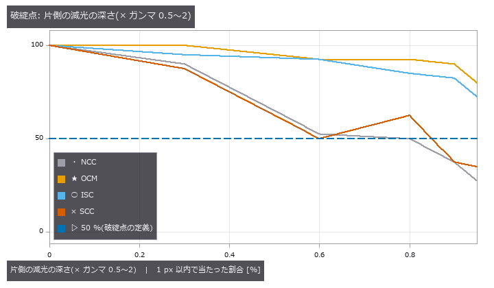
↑ 公開の実写 5 枚から切った 32 x 32 のテンプレートを、雑音 σ = 0.01 の場面で探す。
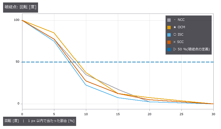
↑ 公開の実写 5 枚から切った 32 x 32 のテンプレートを、雑音 σ = 0.01 の場面で探す。

↑ 空の平坦な所(標準偏差 < 0.01)を切ったテンプレート。

↑ 雑音の無い場面の増分 Δ と σ から、組ごとの一致確率 Φ(Δ/(√2σ)) が決まる。
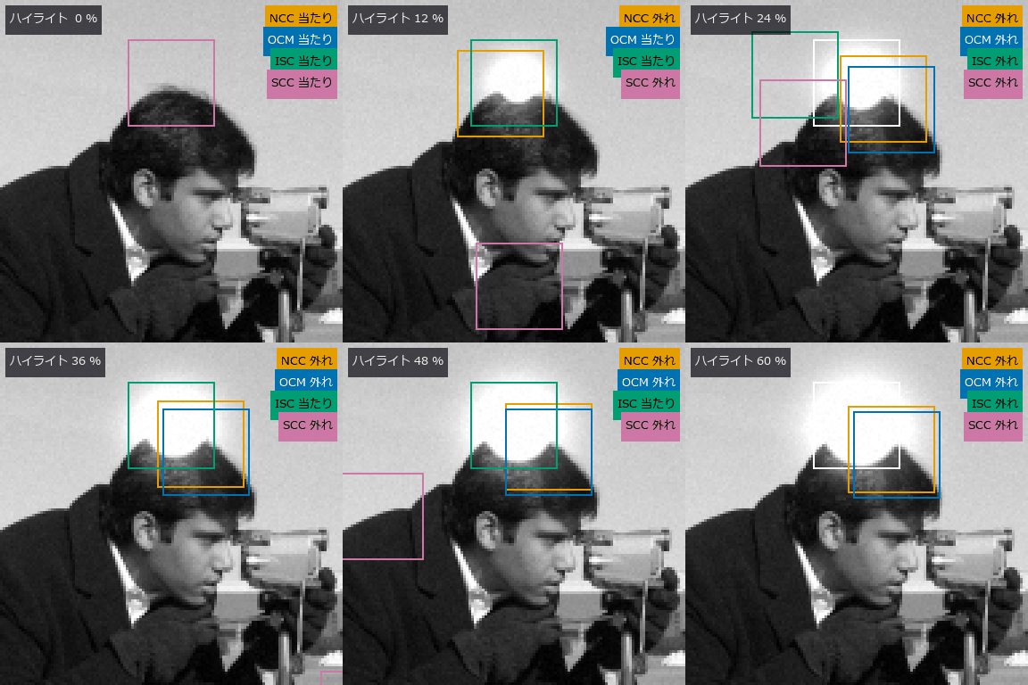
↑ The animation ―― 飽和したハイライトを 0 → 60 % まで広げる(camera、CC0)。白 = 正解、橙 = NCC、青 = OCM、緑 = ISC、紫 = SCC。NCC は最初の数コマで光の縁へ飛ぶ。
py -3.11 examples/poc_code_matching_breakdown.py
Source: examples/poc_code_matching_breakdown.py
This run produced 10 figures in total - see them all
Ops used (notes): isc_match · ncc_locate · ocm_match · radial_reach_filter · reflect · scc_match · text_box
No.2026.256 —— Flagging What Differs from Aligned Good Samples — a Variation Model with a Declared False-Alarm Rate, and Where Real Images Break It
A classic inspection learns the usual per-pixel variation from good parts and flags what falls outside. Here the band is set by a false-alarm rate declared in advance and scored on 200 public real images. Alignment mattered more than the number of good parts, and the declared rate was not kept.

↑ Flagging What Differs from Aligned Good Samples — a Variation Model with a Declared False-Alarm Rate, and Where Real Images Break It ―― The inspection classic, learning every pixel’s usual value and spread from many good samples and flagging what leaves the band, as an op family whose band width is derived from a declared per-pixel false-alarm rate instead of being set by hand (five new varmodel_ ops plus four method-independent anomeval metrics). For normal good samples a new pixel’s deviation follows a t prediction interval, so the band width is closed-form. False-alarm rates counted on synthetic good samples fall inside the binomial 4-sigma band for per-pixel std, one pooled variance, empirical-Bayes shrinkage (Smyth 2004) and median/MAD, and the pooled variance fails when the noise differs per pixel. With five good samples the std band is 9.4 sigma wide (the t4 tail); shrinkage brings it to 5.0 and lifts the detection of 5-sigma flaws from 0.13 to 0.52. A good set shifted by 1-2 px is refused; forced through, the band on edges grows 22-fold and misses every edge flaw, and registering by a 1/20-px Fourier shift brings it back to 1.07. With three of twenty “good” samples carrying the same flaw, std misses the real flaw there (0.00) while median/MAD finds it (0.98). On the public VisA pcb1 data (CC BY 4.0, 200 test images) the registered band reaches pixel AUROC 0.808 and AUPRO 0.678 against 0.705 and 0.460 unregistered; golden comparison scores a higher pixel AUROC (0.826) but a lower AUPRO (0.519). The declared 1e-3 false-alarm rate is not kept on real images (3.8 %), and recalibrating on held-out good images only reaches 2.4 %: a difference between the training and test captures remains that a translation cannot remove. A stochastic texture (DAGM 2007, CC BY 4.0) has no structure in its mean image, its alignment is reported as unobservable and detection is at chance (pixel AUROC 0.465): where the method works and where it does not, both in numbers.*

↑ The measurement ―― 20 枚の良品のうち 3 枚の同じ場所(右上の四角)に +0.3 の傷。std は傷を良品のばらつきとして覚え、帯が太る(左上)ので、同じ場所の本物の傷(+0.2 = 雑音の 10 倍)の z が小さい。中央値と MAD は 3 枚の外れを無視する。左下の傷は汚れていない場所の対照。 (figure labels are in Japanese; the numbers are the same)

↑ VisA pcb1 の試験 200 枚(CC BY 4.0)。

↑ VisA pcb1(CC BY 4.0、灰色・1/4 縮小、欠陥の周りを切り出し、基板の印字は入れない)。

↑ 画素ごとに独立な正規の良品(合成)。
py -3.11 examples/poc_good_sample_variation_model.py
Source: examples/poc_good_sample_variation_model.py
This run produced 5 figures in total - see them all
Ops used (notes): anomaly_image_auroc · anomaly_pixel_auroc · anomaly_pro · anomaly_region_overlap · dc_rpca_sparse · varmodel_alignment · varmodel_calibrate · varmodel_fit · varmodel_score
No.2026.264 —— Anomaly Detection from Good Samples Only — Classical Patch Features, a Per-Position Distribution Against a Memory Bank on One Yard-Stick, Down to a Recall-Guaranteeing Threshold
The most common family in inspection research, learning the features of good samples and flagging patches that leave them, built with classical features (multi-resolution gradients, Gabor, rotation-invariant LBP, spectral bands, colour) instead of a deep network, with the variants compared on one yard-stick (pixel AUROC (area under the ROC curve), AUPRO (area under the per-region-overlap curve), image AUROC, F1 max). Eight new ops: patch_features, patchdist_fit / patchdist_score, patchbank_fit / patchbank_score, and the evaluation additions anomaly_pixel_f1_max, anomaly_image_f1_max and anomaly_operating_point. On a synthetic stochastic texture (smooth random fields with planted spots and thin scratches) the per-position normal distribution scores an AUPRO of 0.375 with 20 good images and loses to the pooled distribution (0.559) and a 10 % memory bank (0.603), in the same order at 5, 20 and 80 good images: it estimates 51 dimensions from few samples per position. Where n <= D makes the covariance singular the shrinkage is declared (intensity 0.374 at 5 good images, 0.067 at 80) and an undeclared one is refused. The existing variation model scores a pixel AUROC of 0.785 on the texture (the memory bank 0.881) and is refused on a weave whose phase differs every time. A logical anomaly, a vertical bar moved by 24 px, is missed by a memory that ignores position (anomaly score 0.9 times that of good images) and found when a position weight is added (3.9 times). Thinning the memory to 10 % keeps AUPRO at 0.638 against 0.684 and cuts the scoring CPU time from 12.55 s to 0.84 s. The operating point that guarantees recall 0.8 at confidence 0.9 keeps its promise in 0.957 of 300 repetitions of the calibrate-on-30-defects procedure, against 0.503 for simply taking the 80 % point of the calibration defects, at the price of more false alarms (0.369 against 0.211). On the public DAGM 2007 Class1 data (a stochastic texture, CC BY 4.0) the variation model scores a pixel AUROC of 0.436, below chance; a gradient-only memory bank reaches 0.768 (AUPRO 0.474) but its per-image AUROC is 0.53, and growing the feature to 51 dimensions drops it to 0.623. On VisA pcb1 (CC BY 4.0, 20 good images) the 10 % memory bank reaches pixel AUROC 0.990, AUPRO 0.875 and image AUROC 0.935 (the variation model: 0.808 and 0.678), and adding the position weight lowers it to 0.969 and 0.790; candle scores 0.895 and 0.734.
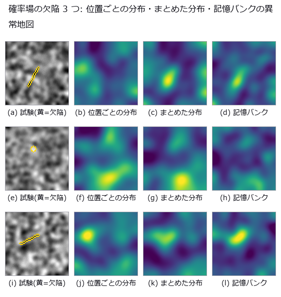
↑ Anomaly Detection from Good Samples Only — Classical Patch Features, a Per-Position Distribution Against a Memory Bank on One Yard-Stick, Down to a Recall-Guaranteeing Threshold ―― The most common family in inspection research, learning the features of good samples and flagging patches that leave them, built with classical features (multi-resolution gradients, Gabor, rotation-invariant LBP, spectral bands, colour) instead of a deep network, with the variants compared on one yard-stick (pixel AUROC (area under the ROC curve), AUPRO (area under the per-region-overlap curve), image AUROC, F1 max). Eight new ops: patch_features, patchdist_fit / patchdist_score, patchbank_fit / patchbank_score, and the evaluation additions anomaly_pixel_f1_max, anomaly_image_f1_max and anomaly_operating_point. On a synthetic stochastic texture (smooth random fields with planted spots and thin scratches) the per-position normal distribution scores an AUPRO of 0.375 with 20 good images and loses to the pooled distribution (0.559) and a 10 % memory bank (0.603), in the same order at 5, 20 and 80 good images: it estimates 51 dimensions from few samples per position. Where n <= D makes the covariance singular the shrinkage is declared (intensity 0.374 at 5 good images, 0.067 at 80) and an undeclared one is refused. The existing variation model scores a pixel AUROC of 0.785 on the texture (the memory bank 0.881) and is refused on a weave whose phase differs every time. A logical anomaly, a vertical bar moved by 24 px, is missed by a memory that ignores position (anomaly score 0.9 times that of good images) and found when a position weight is added (3.9 times). Thinning the memory to 10 % keeps AUPRO at 0.638 against 0.684 and cuts the scoring CPU time from 12.55 s to 0.84 s. The operating point that guarantees recall 0.8 at confidence 0.9 keeps its promise in 0.957 of 300 repetitions of the calibrate-on-30-defects procedure, against 0.503 for simply taking the 80 % point of the calibration defects, at the price of more false alarms (0.369 against 0.211). On the public DAGM 2007 Class1 data (a stochastic texture, CC BY 4.0) the variation model scores a pixel AUROC of 0.436, below chance; a gradient-only memory bank reaches 0.768 (AUPRO 0.474) but its per-image AUROC is 0.53, and growing the feature to 51 dimensions drops it to 0.623. On VisA pcb1 (CC BY 4.0, 20 good images) the 10 % memory bank reaches pixel AUROC 0.990, AUPRO 0.875 and image AUROC 0.935 (the variation model: 0.808 and 0.678), and adding the position weight lowers it to 0.969 and 0.790; candle scores 0.895 and 0.734.
Terms: AUROC — The area under the receiver-operating-characteristic curve, summarizing ranking performance across thresholds on a 0-to-1 scale.; ROC — A curve of true-positive rate against false-positive rate as the decision threshold varies, showing a binary detector’s trade-off.; AUPRO — An anomaly-localization metric integrating per-region overlap against false-positive rate over a specified false-positive range.
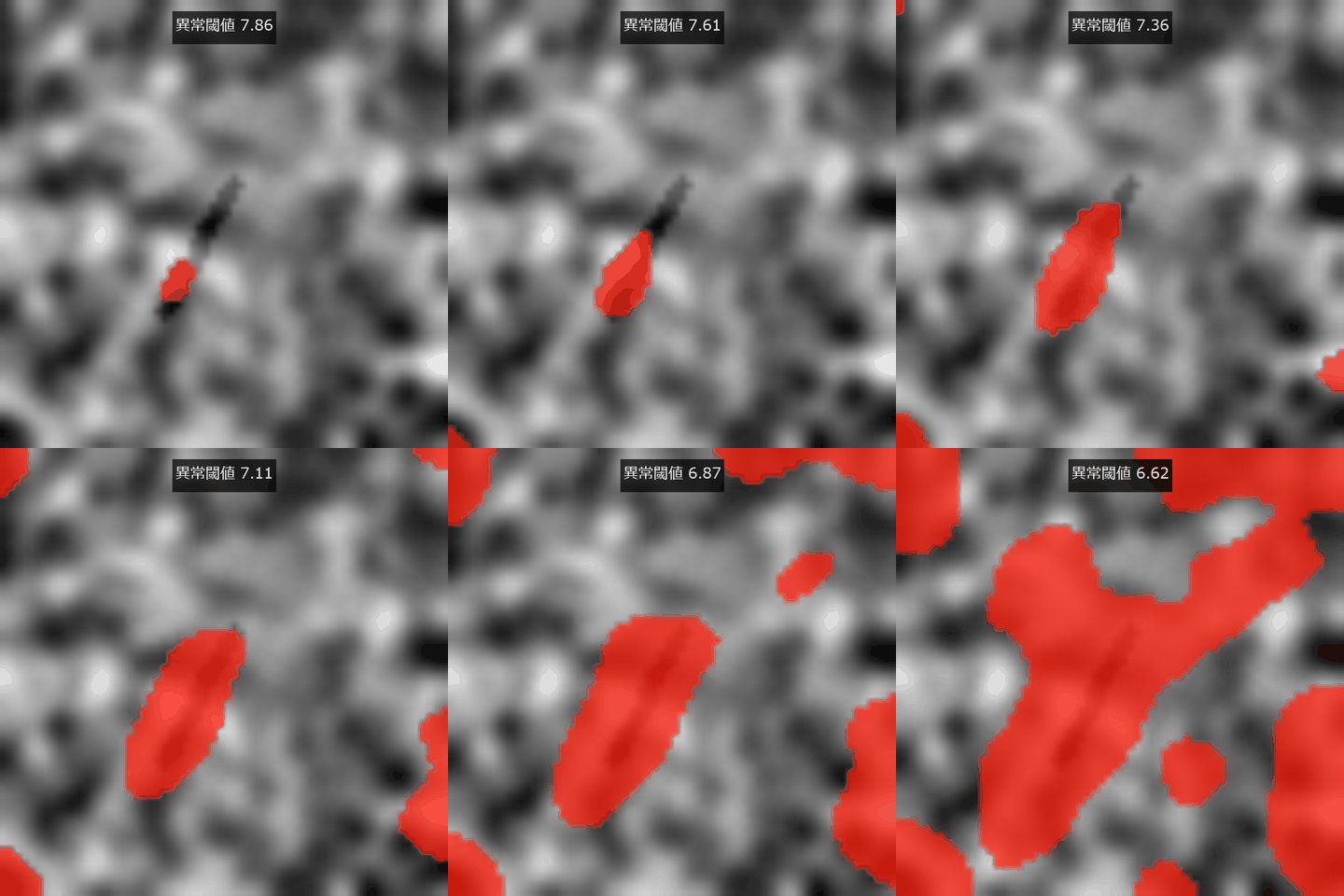
↑ The measurement ―― 記憶バンクの異常度閾値を下げると欠陥領域が現れる。 (figure labels are in Japanese; the numbers are the same)
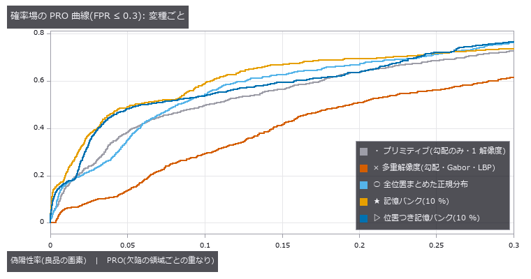
↑ 確率場・良品 20 枚の PRO 曲線。
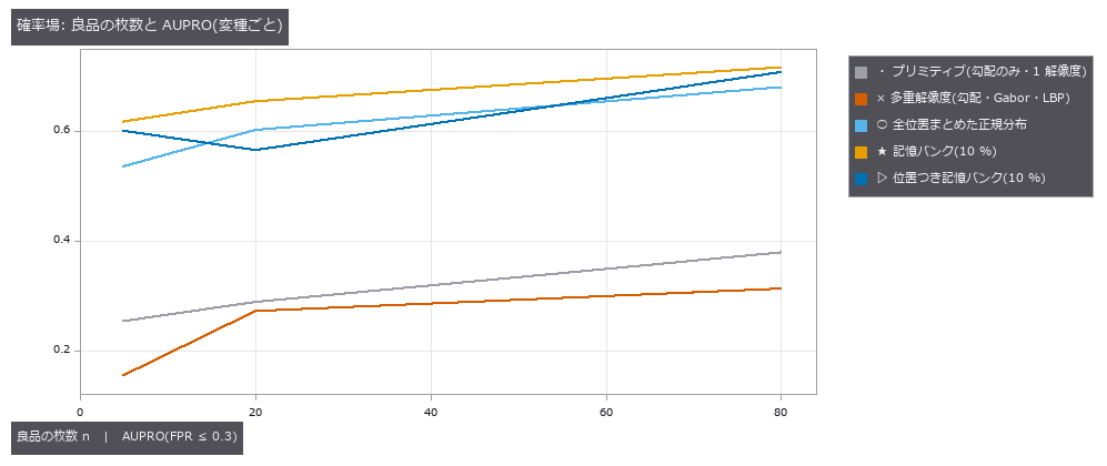
↑ 確率場の試験画像での AUPRO。
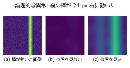
↑ 良品では縦の棒は左(x = 20)にある。
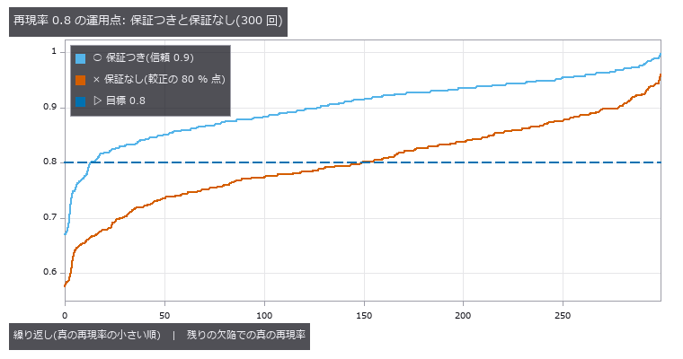
↑ 欠陥 400 枚のプールから較正に欠陥 30 枚を引いて閾値を決め、残りの欠陥で真の再現率を測った 300 回を小さい順に並べた。
py -3.11 examples/poc_patch_anomaly.py
Source: examples/poc_patch_anomaly.py
This run produced 11 figures in total - see them all
Ops used (notes): anomaly_image_auroc · anomaly_operating_point · anomaly_pixel_auroc · anomaly_pixel_f1_max · anomaly_pro · anomaly_region_overlap · gabor · intensity · patch_features · patchbank_fit · patchbank_score · patchdist_fit · varmodel_fit · varmodel_score
No.2026.258 —— Counting Dense Bubbles — When the Overlap Is Too Deep to Decide, Return an Interval Instead of a Count
Overlapping bubbles show up as peaks of the distance transform, and as the neck between them gets shallower the image stops deciding whether there are two bubbles or one. The existing chain (blob_distance, blob_seeds, blob_split) picks one h and always returns one number, so it calls two circles at overlap 0.8 a single bubble. The new op blob_count_interval measures each peak’s prominence (0-dimensional persistence), returns an interval when the relative prominence falls inside a band, and opens the upper bound when the inscribed circles of the counted peaks cannot explain the area. The relative prominence of two equal circles follows the closed form 1 − sqrt(1 − (1 − o)²) to within 1.6 px, and upscaling by 2 leaves every answer unchanged. Confident errors appear only beyond the overlap where the union becomes indistinguishable from an ellipse of aspect 1.1 (0.86 to 0.90 by the closed form). On the BBBC005 ground-truth masks (CC0) the small objects are counted with a relative error of 0.34 % (connected components 9.4 %); for the deeply overlapping large objects the op declines to give a number on 286 of 300 images and makes no confident error. Semi-synthetic clusters built from real oxygen-bubble shapes of a water electrolyser (PEMWE, CC BY 4.0, hand-drawn masks) give 2 confident errors in 65 scenes and an ALCON2009-style score (centroid inside each bubble’s box, implemented here) of 0.95 on the clusters it answers. Widening the shape tolerance until 95 % of isolated bubbles pass lets hidden bubbles through and raises the error rate from 3 % to 19 % — the sweep shows the trade-off between counting more and never being silently wrong. When irregular bubbles overlap deeply, even the upper bound of the declined interval can miss by one; the op documents this limit.

↑ Counting Dense Bubbles — When the Overlap Is Too Deep to Decide, Return an Interval Instead of a Count ―― Overlapping bubbles show up as peaks of the distance transform, and as the neck between them gets shallower the image stops deciding whether there are two bubbles or one. The existing chain (blob_distance, blob_seeds, blob_split) picks one h and always returns one number, so it calls two circles at overlap 0.8 a single bubble. The new op blob_count_interval measures each peak’s prominence (0-dimensional persistence), returns an interval when the relative prominence falls inside a band, and opens the upper bound when the inscribed circles of the counted peaks cannot explain the area. The relative prominence of two equal circles follows the closed form 1 − sqrt(1 − (1 − o)²) to within 1.6 px, and upscaling by 2 leaves every answer unchanged. Confident errors appear only beyond the overlap where the union becomes indistinguishable from an ellipse of aspect 1.1 (0.86 to 0.90 by the closed form). On the BBBC005 ground-truth masks (CC0) the small objects are counted with a relative error of 0.34 % (connected components 9.4 %); for the deeply overlapping large objects the op declines to give a number on 286 of 300 images and makes no confident error. Semi-synthetic clusters built from real oxygen-bubble shapes of a water electrolyser (PEMWE, CC BY 4.0, hand-drawn masks) give 2 confident errors in 65 scenes and an ALCON2009-style score (centroid inside each bubble’s box, implemented here) of 0.95 on the clusters it answers. Widening the shape tolerance until 95 % of isolated bubbles pass lets hidden bubbles through and raises the error rate from 3 % to 19 % — the sweep shows the trade-off between counting more and never being silently wrong. When irregular bubbles overlap deeply, even the upper bound of the declined interval can miss by one; the op documents this limit.

↑ The measurement ―― 等しい 2 円の 2 番目の山の相対突出度。閉形式(破線)は半径によらない。実測は格子の量子化で閉形式より最大 1.5 px 低い。点線の帯の中に落ちた山は『あいまい』。 (figure labels are in Japanese; the numbers are the same)
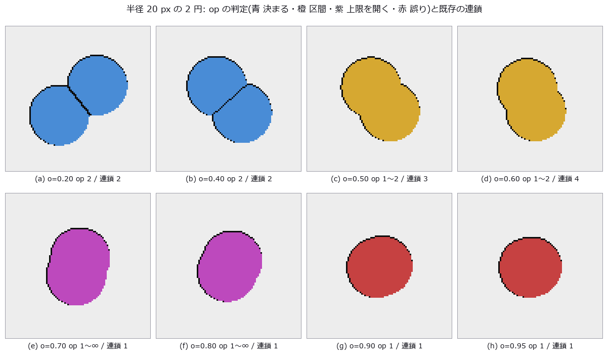
↑ 重なり率を上げると、くびれが浅くなって 0.5 前後で『1 個か 2 個か』が決まらなくなり(橙)、0.7 を超えると山が 1 つになる。

↑ world_blobs_touching(12 円、半径 14 px)。

↑ BBBC005 の真値マスク。
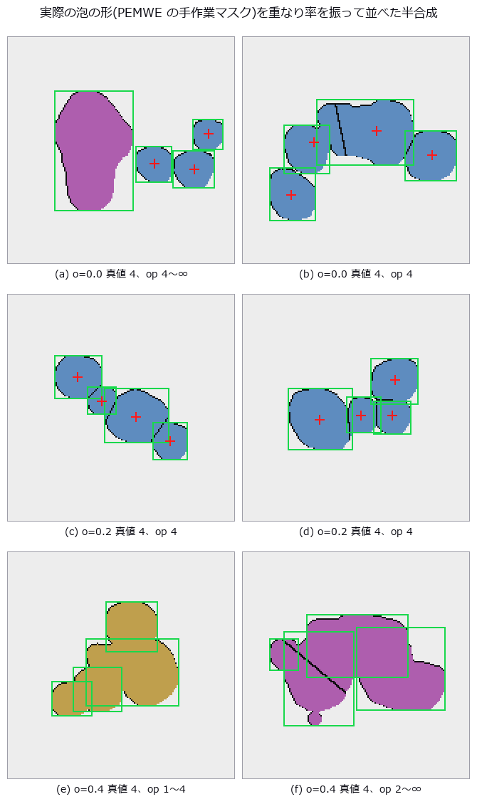
↑ 緑の矩形 = 置いた泡(真値)、赤の十字 = 決まった塊の重心。
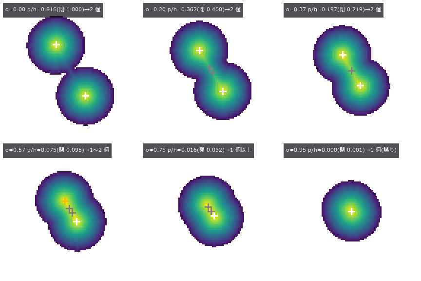
↑ The animation ―― 2 つの泡が近づいて融合していく。色 = 距離変換(内接円の半径)、白い十字 = 確かな山、橙 = あいまいな山。くびれが浅くなると 2 番目の山が帯に落ち、やがて消える。
py -3.11 examples/poc_dense_bubble_count.py
Source: examples/poc_dense_bubble_count.py
This run produced 12 figures in total - see them all
Ops used (notes): blob_count_interval · blob_distance · blob_features · blob_label · blob_seeds · blob_split · text_box · world_blobs_touching
No.2026.280 —— Fourier Ptychography — 20x-Equivalent Resolution and Phase from a 4x Objective’s Wide Field, by Iterative Phase Retrieval
A low-magnification objective sees a wide field but misses fine detail. Combining images lit from different angles in frequency space resolved detail as fine as a 20x image over the same wide field. When the illumination overlap is too small to converge, no answer is returned.

↑ Fourier Ptychography — 20x-Equivalent Resolution and Phase from a 4x Objective’s Wide Field, by Iterative Phase Retrieval ―― Keep the wide field of a low-magnification objective, take a set of images under LED illumination from many angles, stitch them in frequency space and recover a 20x-equivalent resolution and the phase by iterative phase retrieval. Six new ops (fourierptycho, category fpm of opsoptics): closed-form design numbers before measuring (synthetic NA, cut-off period, pupil overlap, LED count, sampling, LEDs on the bright-/dark-field boundary), a USAF target, a capture simulator (noise, aberrations, LED misalignment, reflective heights), an entry point for measured data, a reconstruction with joint pupil recovery and LED position correction that returns its convergence history, stop reason and synthetic NA and refuses unless it converges, and an element-by-element USAF read-out. With a 4x / NA 0.1 objective and 13 x 13 LEDs (synthetic NA 0.424) one image resolves G7 E4 (5.53 um; closed form 5.32 um) and FP resolves G9 E5 (1.22 um; closed form 1.25 um), the same element as a 20x / NA 0.40 coherent image. Phase within 0.13 rad rms of the band-limited truth; reflective 20-40 nm steps within 4.0 nm rms. Lowering the pupil overlap from 64 % to 7 %, 43 % and above converge while 32 % and below are refused, bracketing the published 35 % minimum; the residual alone cannot tell (18 % overlap has a smaller residual than 64 %). Pupil aberrations of 0.12 waves rms are recovered to 0.005 waves and an LED array offset of (0.6, -0.4) mm, 1 deg and 1.5 mm is read back as (0.62, -0.36) mm, 0.93 deg and 1.25 mm. Flipping the sign of k yields the phase-conjugate image with the same residual. On public FP data of a USAF target (not shipped; run only when present) FP resolves G9 E3 (1.55 um) against the closed-form 1.60 um from the published set-up; a single raw image resolves G7 E3. Nothing learned, nothing calibrated, 33 gates.

↑ The measurement ―― G9(周期 1.95〜1.06 µm)を 3 倍に拡大。FP は E5(1.22 µm)まで 3 本の棒が分かれる。 (figure labels are in Japanese; the numbers are the same)
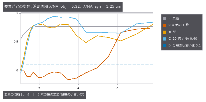
↑ この回の図
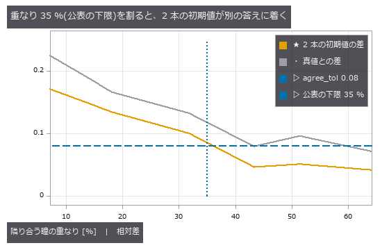
↑ この回の図
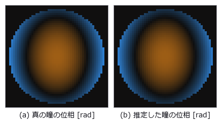
↑ 瞳の円(NA 0.1)の中の位相。
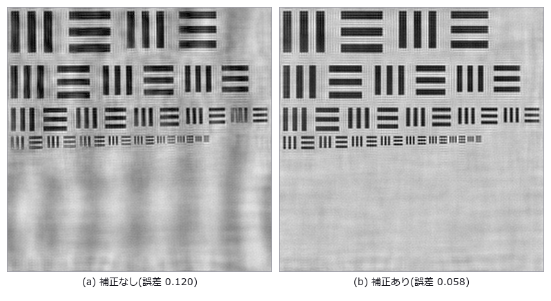
↑ LED アレイが (0.6, −0.4) mm・1°・高さ 1.5 mm ずれている。
py -3.11 examples/poc_fourier_ptychography.py
Source: examples/poc_fourier_ptychography.py
This run produced 11 figures in total - see them all
Ops used (notes): coherent_image · fp_capture · fp_design · fp_element_contrast · fp_reconstruct · fp_stack_from_images · fp_usaf_target
No.2026.281 —— Sorting Multi-Robot Plans with the Same Starts and Goals by How They Wind — Counting Homotopy Classes with Space-Time Braids and Dynnikov Coordinates, 61 Planner Candidates in 26 Classes
Stack moving vehicles and fixed pillars along time and you get a braid; two plans that deform into each other with their ends held fixed are exactly the plans with the same braid. The times at which neighbouring strands swap order along a projection axis are solved in closed form into a signed crossing sequence (a braid word), and three independent deciders — Dynnikov coordinates, Dehornoy handle reduction and the Artin representation — decide whether two words are the same braid (background: homotopy in planar multi-agent path planning, doi:10.1613/jair.1.19243). The figure spins three differently wound plans of three robots as space-time braids. Gates: the braid relations hold under the Dynnikov action in 1311 cases with integer error 0 and real error 2.8e-14, while the non-relation σ₁σ₂ = σ₂σ₁ breaks in 100/100. The three deciders agree on 100/100 equal and 100/100 different braids; Dynnikov coordinates match the MIT-licensed reference implementation in 240/240. One robot around a pillar: shortest cost per class [14, 14, 30, 30, 46] = closed form 14 + 16m. 61 candidates from the agvfleet planners (CBS + prioritised with waypoints) fall into 26 classes, and the CBS optimum 40 represents the cheapest one. A commutator a b a⁻¹ b⁻¹ has all windings 0 yet a non-trivial braid. Trap: point-symmetric grid moves create projection triple points that no change of angle removes — a tiny constant per-strand offset resolves them. Honestly: there are infinitely many classes, and only those the candidate sampler finds are listed (waypoint sampling found 3 of 8).
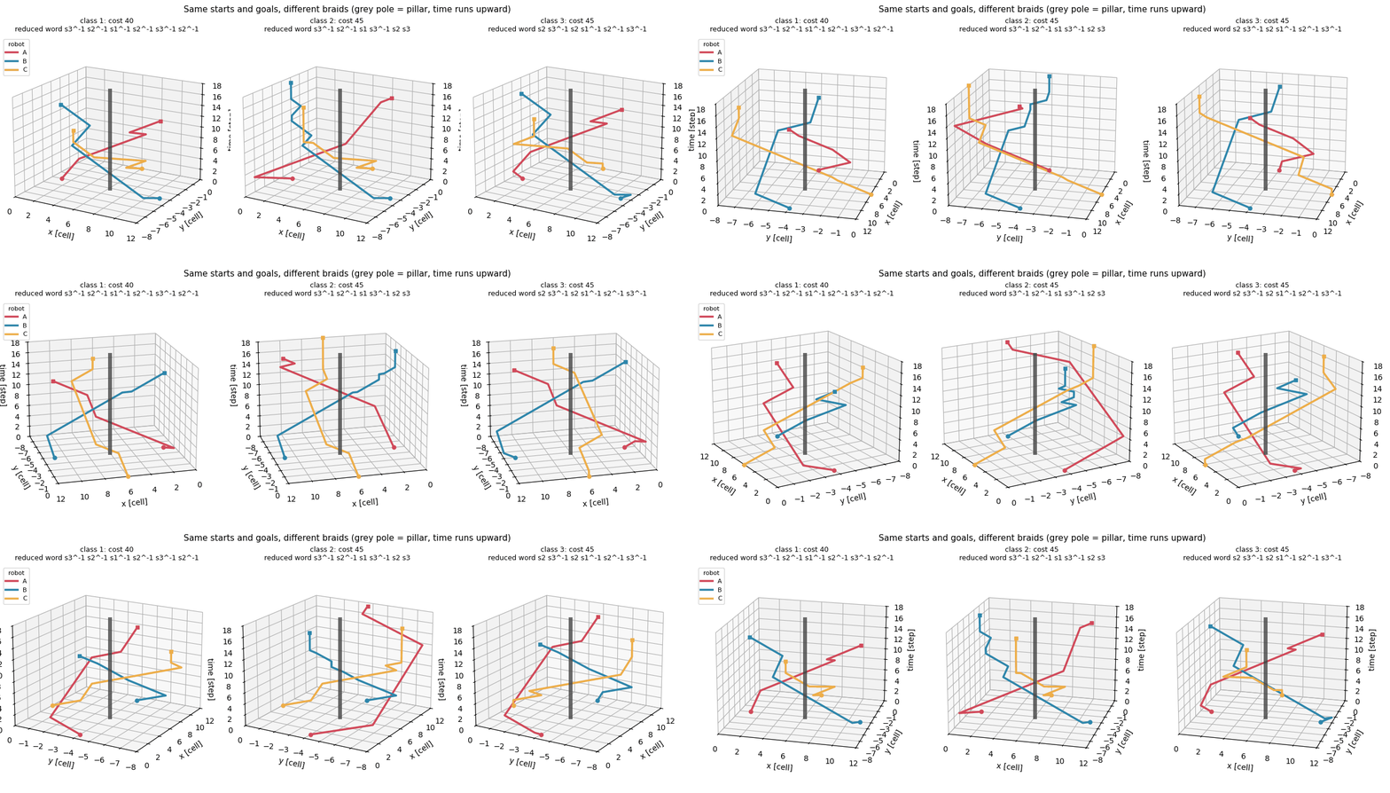
↑ Sorting Multi-Robot Plans with the Same Starts and Goals by How They Wind — Counting Homotopy Classes with Space-Time Braids and Dynnikov Coordinates, 61 Planner Candidates in 26 Classes ―― Stack moving vehicles and fixed pillars along time and you get a braid; two plans that deform into each other with their ends held fixed are exactly the plans with the same braid. The times at which neighbouring strands swap order along a projection axis are solved in closed form into a signed crossing sequence (a braid word), and three independent deciders — Dynnikov coordinates, Dehornoy handle reduction and the Artin representation — decide whether two words are the same braid (background: homotopy in planar multi-agent path planning, doi:10.1613/jair.1.19243). The figure spins three differently wound plans of three robots as space-time braids. Gates: the braid relations hold under the Dynnikov action in 1311 cases with integer error 0 and real error 2.8e-14, while the non-relation σ₁σ₂ = σ₂σ₁ breaks in 100/100. The three deciders agree on 100/100 equal and 100/100 different braids; Dynnikov coordinates match the MIT-licensed reference implementation in 240/240. One robot around a pillar: shortest cost per class [14, 14, 30, 30, 46] = closed form 14 + 16m. 61 candidates from the agvfleet planners (CBS + prioritised with waypoints) fall into 26 classes, and the CBS optimum 40 represents the cheapest one. A commutator a b a⁻¹ b⁻¹ has all windings 0 yet a non-trivial braid. Trap: point-symmetric grid moves create projection triple points that no change of angle removes — a tiny constant per-strand offset resolves them. Honestly: there are infinitely many classes, and only those the candidate sampler finds are listed (waypoint sampling found 3 of 8).

↑ The measurement ―― 図 01 の最初のコマ(等倍・可逆 PNG)。 (figure labels are in Japanese; the numbers are the same)

↑ 同じ 3 つの計画を床の上から見る(× は柱の代表の点)。

↑ 1 台が柱を避けて左から右へ: 類ごとの最短経路を短い順に 5 本(費用 14・14・30・30・46 = 14 + 16m)。

↑ 候補を類に分けた表(費用の安い順)。
py -3.11 examples/poc_braid_homotopy_classes.py
Source: examples/poc_braid_homotopy_classes.py
This run produced 5 figures in total - see them all
Ops used (notes): braid_class_representatives · braid_equivalent · braid_from_trajectories · braid_reduce · dynnikov_act · dynnikov_coordinates · grid_distances · grid_hole_points · grid_paths_to_xy · homotopy_class_compare · homotopy_shortest_paths · mapf_cbs · mapf_prioritized · pairwise_winding · plan_conflicts · plan_cost
No.2026.282 —— The Marechal Approximation Breaks at Different RMS Errors for Different Aberration Shapes
Four Noll-normalised aberrations are swept over 484 conditions. Fixed-axis intensity ratio, same-plane peak ratio and peak location are defined separately. Coma at 0.2/0.3 waves gives fixed-axis ratios 0.1816/0.0127, peak ratios 0.2178/0.1437 and peak shifts of 8/17 pixels. The 5 percent Marechal boundaries quoted are for the fixed-axis definition. Mahajan (1982/1983) already reported aberration-specific results; this PoC is a definition and implementation reproduction.
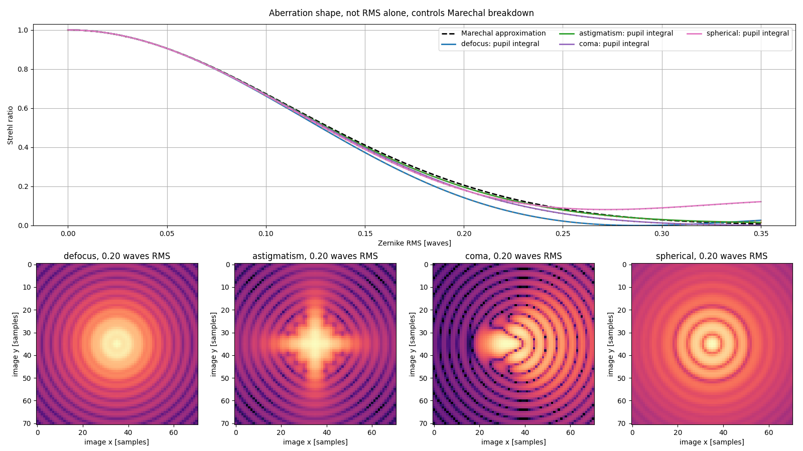
↑ The Marechal Approximation Breaks at Different RMS Errors for Different Aberration Shapes ―― Four Noll-normalised aberrations are swept over 484 conditions. Fixed-axis intensity ratio, same-plane peak ratio and peak location are defined separately. Coma at 0.2/0.3 waves gives fixed-axis ratios 0.1816/0.0127, peak ratios 0.2178/0.1437 and peak shifts of 8/17 pixels. The 5 percent Marechal boundaries quoted are for the fixed-axis definition. Mahajan (1982/1983) already reported aberration-specific results; this PoC is a definition and implementation reproduction.
py -3.11 examples/poc_wavefront_aberration_limits.py
Source: examples/poc_wavefront_aberration_limits.py
This run produced 1 figures in total - see them all
Ops used (notes): pupil_psf
No.2026.283 —— A Four-Angle Polarization Camera Leaves Seven Mueller (4-by-4 polarization-transfer matrix) Dimensions Unseen
The design matrix formed by 0, 45, 90 and 135 degree linear micro-analysers has SVD-computed rank 9 of 16; the number is not hard-coded. Adding quarter-wave-plate states on generation and analysis raises the rank to 16. Fullseye’s Mueller chain and an independent Kronecker design equation agree within 1.39e-17. Across 200 trials with 0.2 percent read noise, median relative Mueller error falls from 41.64 percent for linear-only measurements to 1.40 percent with the QWP states.
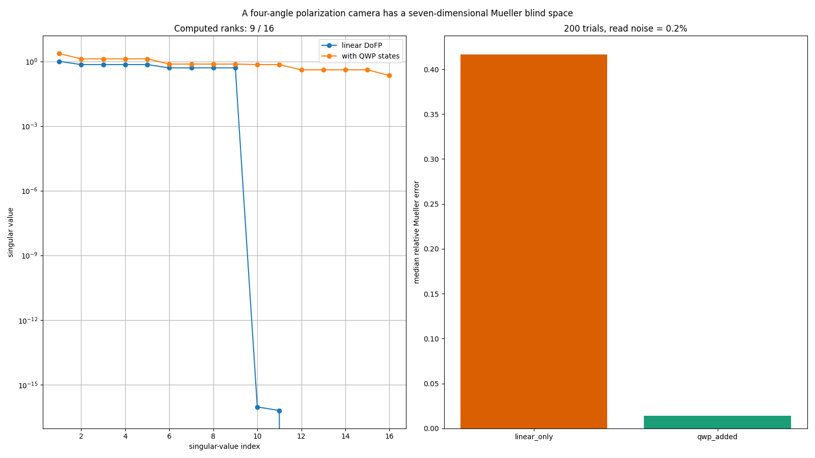
↑ A Four-Angle Polarization Camera Leaves Seven Mueller (4-by-4 polarization-transfer matrix) Dimensions Unseen ―― The design matrix formed by 0, 45, 90 and 135 degree linear micro-analysers has SVD-computed rank 9 of 16; the number is not hard-coded. Adding quarter-wave-plate states on generation and analysis raises the rank to 16. Fullseye’s Mueller chain and an independent Kronecker design equation agree within 1.39e-17. Across 200 trials with 0.2 percent read noise, median relative Mueller error falls from 41.64 percent for linear-only measurements to 1.40 percent with the QWP states.
Terms: Mueller matrix — A real 4-by-4 matrix acting on a Stokes vector to describe how an optical element or sample changes polarization.
py -3.11 examples/poc_mueller_dofp_observability.py
Source: examples/poc_mueller_dofp_observability.py
This run produced 1 figures in total - see them all
Ops used (notes): mueller_element
No.2026.284 —— Slanted-Edge SFR Misreads MTF50 (spatial frequency at 50% MTF) Through Gamma as Well as Edge Angle
For a 3.45 um pixel, F/5.6 and 550 nm system, the circular-pupil Airy OTF is applied to a high-resolution edge before pixel-area integration, so forward model and truth agree over the full frequency range. Central-difference correction is 1 at DC and 1.1107207 at Nyquist. Across 420 conditions the remaining clean linear estimator error is at most 0.00872 cycles per pixel, displayed separately from zero model error; failures beyond 10 percent begin at 1.0 degree.

↑ Slanted-Edge SFR Misreads MTF50 (spatial frequency at 50% MTF) Through Gamma as Well as Edge Angle ―― For a 3.45 um pixel, F/5.6 and 550 nm system, the circular-pupil Airy OTF is applied to a high-resolution edge before pixel-area integration, so forward model and truth agree over the full frequency range. Central-difference correction is 1 at DC and 1.1107207 at Nyquist. Across 420 conditions the remaining clean linear estimator error is at most 0.00872 cycles per pixel, displayed separately from zero model error; failures beyond 10 percent begin at 1.0 degree.
Terms: MTF50 — The spatial frequency at which MTF falls to 50% of its low-frequency value, used as a single-number resolution summary.; MTF — The magnitude of the optical transfer function, showing how image contrast is transferred at each spatial frequency.; Nyquist — The highest frequency a sampling grid can represent: half a cycle per sample. Finer patterns fold back and appear as a different, coarser pattern.
py -3.11 examples/poc_slanted_edge_sfr_limits.py
Source: examples/poc_slanted_edge_sfr_limits.py
This run produced 1 figures in total - see them all
Ops used (notes): mtf_diffraction
The Dimensional and Shape Metrology Wing — Keep Bias and Scatter Apart
To state that a part is 50.50 pixels wide, you need bias (the part that always shifts the same way) and scatter (the part that changes from shot to shot) as two separate numbers. Pass/fail is decided by bias; repeatability by scatter. Merge them into one ‘error’ and you no longer know which countermeasure to take.
The 45 exhibits here hold their ground truth in closed form or analytic rendering — a signed-distance-function part, an involute gear, a roughness surface synthesised from a prescribed PSD, a white-light interferometry stack, analytic speckle, Frocht’s stress field, a perfectly symmetric synthetic skull — and then score caliper, correlation and phase readings against it.
The recurring finding is that a number without its definition cannot be compared: crack widths that differ by 0.20 mm between two distance-transform conventions, a D50 that differs by 1.66x between number- and area-weighting, an Sz that never plateaus as the evaluation area grows, an orientation index that moves 5 % depending on whether the truth is counted by fibre or by length. These are not instrument errors; they are questions of what you are comparing against.
No.2026.120 —— Matching Full 2-D Inspection to Sampled 3-D Inspection — A Grid Overlaps Itself
Full visual inspection and sampled CT must assign the same index to each joint. Unequal-sided fiducials fixed this correspondence, then top-ranked candidates caught 19 % of interface-touching voids. Apparent void rankings can agree while most life-limiting parts are missed.

↑ Matching Full 2-D Inspection to Sampled 3-D Inspection — A Grid Overlaps Itself ―― The real line has two stages: AOI images every unit from above, X-ray CT samples a few and images the inside. What the floor wants to know is how far the CT numbers follow from the AOI numbers — which is not a question about one instrument’s accuracy but about whether two instruments’ indices point at the same joint. A regular array does not match one-to-one on point positions alone: all 30 pads of a 6x5 grid have degenerate distance signatures (9 distinct ones), because the grid maps onto itself and the orientation cannot be read. Fiducials with three distinct side lengths (3600/5200/6325 um) pin rotation and reflection uniquely, and the correspondence is recovered exactly under translation, rotation and re-indexing. With that closed, AOI’s apparent void fraction correlates 0.973 with CT volume fraction and the worst five agree 5/5 — yet of the 27 parts carrying an interface-touching void (the kind that shortens life), those five catch only 19 %. Agreeing on the ranking does not mean catching the dangerous ones. The failed first attempt (Kabsch alone) is kept.
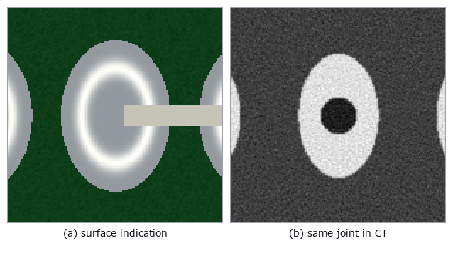
↑ The measurement ―― Matched crop of one joint: surface appearance and internal reconstructed void at the same coordinates. (figure labels are in Japanese; the numbers are the same)

↑ AOI は全数・2-D、CT は抜き取り・3-D。

↑ 直線は「面積率に比例する」という素朴な仮定。
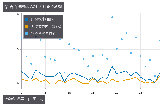
↑ AOI の面積率が大きい接合部が、界面に接するボイドを持つとは限らない。

↑ 同じロットを同じ「悪い順」で並べても、順位は一致しない。
py -3.11 examples/poc_aoi_ct_traceability.py
Source: examples/poc_aoi_ct_traceability.py
This run produced 6 figures in total - see them all
Ops used (notes): filtered_backprojection · radon_transform · vol_label
No.2026.091 —— As-built wall deviation — the bounding box measures the room’s heading, not its size
Point-cloud dimensions can confuse room heading or furniture with wall position. A room with known tilt and bulges was rotated, while its plane-pair error stayed at +2.24 mm. Bounding boxes grow with heading and sample count; plane fitting jumps to furniture when outliers become the majority.
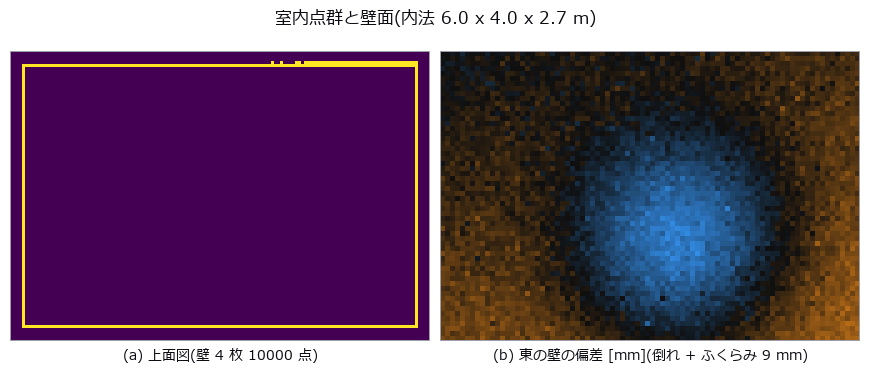
↑ As-built wall deviation — the bounding box measures the room’s heading, not its size ―― A 6.0 x 4.0 x 2.7 m indoor point cloud carries known defects: wall plumb errors of 1.20-9.00 mrad, a 5.00 mrad plan-view squareness error, and a 9 mm out-of-plane bulge. The naive axis-aligned bounding box over-reports the width by 19.1 mm, and rotating the room by just 1 deg relative to the scanner axes adds 80.1 mm (611.1 mm at 10 deg) — it is measuring W cos psi + D sin psi, the room’s heading, while the plane-pair distance stays at +2.24 mm regardless. The AABB also grows with sample size (+14.9 to +19.7 mm for 256x more points, the 2-sigma-sqrt(2 ln N) extreme-value law), so adding measurements makes it worse. Furniture outliers break the two estimators differently: least squares is off by 11x the truth at 10 % contamination (66.3 mrad vs a closed-form 63.8), while RANSAC holds to 45 % and then jumps onto the cabinet at 55 % — where the plumb error stays a harmless 0.13 mrad but the plane itself is 449.9 mm out, so one number hides the failure. A single bulge corrupts plumb (-1.258 mrad), squareness (+0.500 mrad) and the internal dimension (+2.2 mm) at once, all predicted in closed form to within 0.06 mrad.

↑ The measurement ―― 許容 ±10 mm。AABB は ψ=0.5 度で既に外れる。 (figure labels are in Japanese; the numbers are the same)

↑ この回の図
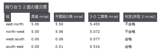
↑ この回の図
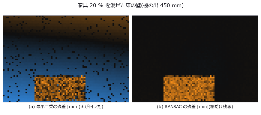
↑ この回の図

↑ この回の図
py -3.11 examples/poc_asbuilt_wall_deviation.py
Source: examples/poc_asbuilt_wall_deviation.py
This run produced 12 figures in total - see them all
Ops used (notes): aabb · angle_between_planes · angle_line_plane · distance_point_plane · fit_plane3 · ransac_plane
No.2026.092 —— Measuring electrode breathing in microns — sub-pixel is not enough
Slight electrode growth must be separated from brightness changes between scans. Layer boundaries were tracked across two cross-sections, recovering a stack increase of +2.136 µm. A fixed brightness crossing reports false strain after an offset, whereas the gradient peak remains at zero.
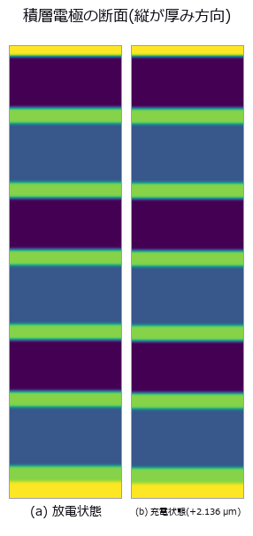
↑ Measuring electrode breathing in microns — sub-pixel is not enough ―― Electrode swelling is read from two cross-sections by tracking layer boundaries to sub-pixel accuracy. Ground truth: anode 1.00 %, cathode 0.20 %, separator 0 %, stack 480.0 -> 482.136 um (+2.136 um = +0.4450 %). Counting binarised pixels resolves 0 of 12 layers, while a fixed-threshold crossing is also sub-pixel and lands on the answer with no noise (+0.004495) — what kills it is the control group: with zero strain, an illumination offset of +0.10 alone yields -1.07e-02, a false strain 2.4x the true one and of the opposite sign, and a gain of x1.30 halves the crossings so the measurement fails outright. The gradient-peak estimator (measure_pos) stays at exactly 0.0 under both. Doubting our own ‘1.8e-14 px error’ and shifting the stack by fractions of a pixel showed that figure to be an artefact of putting the truth on pixel centres: the real error is peak locking, RMS 0.0088 / max 0.0122 px, worth 3.0 % on the anode’s strain. The cliff has two steps, and the one where boundary counts collapse arrives 5.5x earlier than the predicted 3-sigma limit.
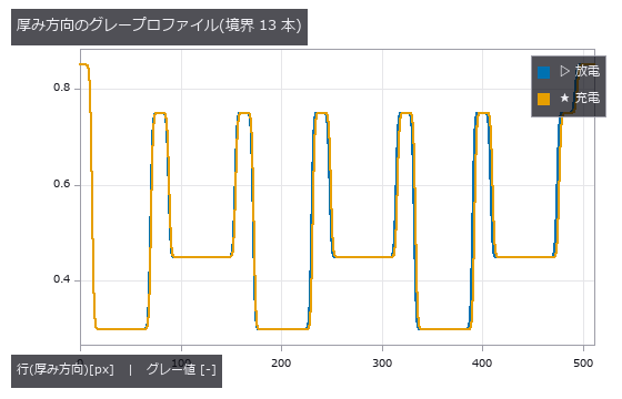
↑ The measurement ―― 境界は erf の重ね合わせで解析的に置いてあるので、真値は浮動小数点の精度で既知。 (figure labels are in Japanese; the numbers are the same)
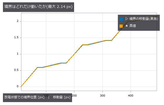
↑ 階段状に増えるのは、伸びる層(負極 1.00 %)と伸びない層(セパレータ 0 %)が交互だから。
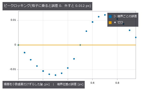
↑ 真値を画素の中心に置いた検査は、推定器を実力以上に良く見せる。
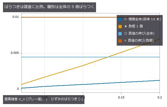
↑ 横線は真値。
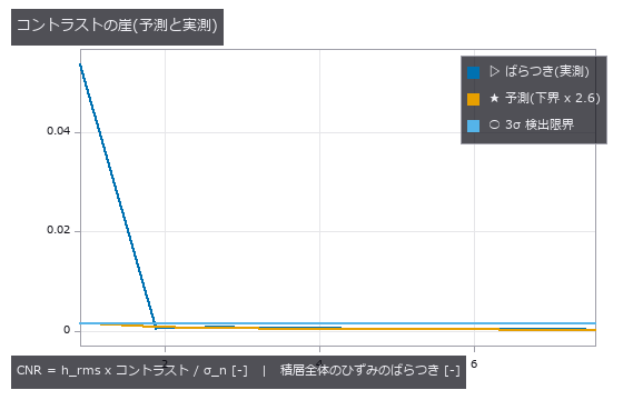
↑ 実測が予測から離れる左端は、雑音が増えたのではなく境界を数え損ねている。
py -3.11 examples/poc_battery_electrode_breathing.py
Source: examples/poc_battery_electrode_breathing.py
This run produced 9 figures in total - see them all
Ops used (notes): auto_threshold · gen_measure_rectangle2 · measure_pos · piv_peak_locking
No.2026.005 —— Measuring Bilateral Asymmetry — The Symmetry Plane Gets Dragged by the Deformation
A reference plane for left-right asymmetry may be pulled toward a one-sided deformation. A known bulge was added to a symmetric skull; the best-fit plane moved by 2.92 mm. The optimized plane shifts toward the bulge and removes part of the asymmetry that should be reported.
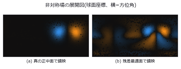
↑ Measuring Bilateral Asymmetry — The Symmetry Plane Gets Dragged by the Deformation ―― A perfectly symmetric synthetic skull with a known bulge added on one side, mirrored and overlaid. Even a perfectly symmetric specimen never scores 0: the floor drops from 1.33 mm (point-to-point) to 0.030 mm (point-to-plane) to 0.012 mm (neighbourhood smoothing). The residual-minimising plane is dragged 2.92 mm / 1.72 degrees by a 6.33 mm bulge, and 46 % of the asymmetry disappears.

↑ The measurement ―― 完全対称な標本を測った残差。点対点は点間隔がそのまま床になる。 (figure labels are in Japanese; the numbers are the same)
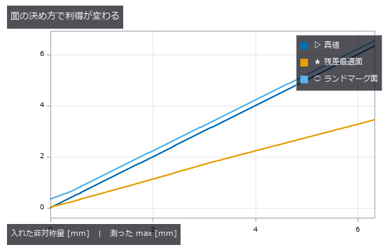
↑ 真値の線は利得 1.0。
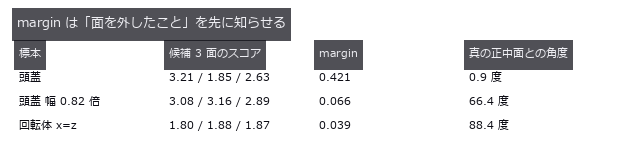
↑ margin < 0.1 で採用を止めれば、66〜88 度の外しは弾ける。
py -3.11 examples/poc_bilateral_asymmetry.py
Source: examples/poc_bilateral_asymmetry.py
This run produced 4 figures in total - see them all
Ops used (notes): chamfer_distance · detect_reflection_symmetry · detect_rotational_symmetry · estimate_normals · hausdorff_distance · reflect_points · reflection_symmetry_score · sample_surface · vertex_normals
No.2026.013 —— Strain From Speckle Images (DIC)
Displacement and strain read from a speckle pair in which 3000 Gaussian spots were moved by the deformation map and redrawn, not interpolated. For a true shift of 0.37 px the window-correlation estimator (piv) is biased by 0.0002 px with 0.0022 px scatter, 167x better than the null that answers ‘no motion’. A rigid rotation manufactures several hundred µε of false strain under the small-strain definition; Green-Lagrange gives exactly 0.
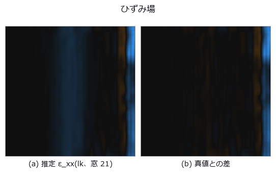
↑ Strain From Speckle Images (DIC) ―― Displacement and strain read from a speckle pair in which 3000 Gaussian spots were moved by the deformation map and redrawn, not interpolated. For a true shift of 0.37 px the window-correlation estimator (piv) is biased by 0.0002 px with 0.0022 px scatter, 167x better than the null that answers ‘no motion’. A rigid rotation manufactures several hundred µε of false strain under the small-strain definition; Green-Lagrange gives exactly 0.
Terms: DIC — A method that correlates local surface patterns before and after deformation to measure displacement and derive strain.
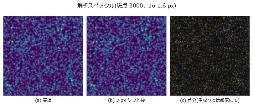
↑ The measurement ―― 変形は補間ではなく斑点の再描画。だから真値が厳密。 (figure labels are in Japanese; the numbers are the same)
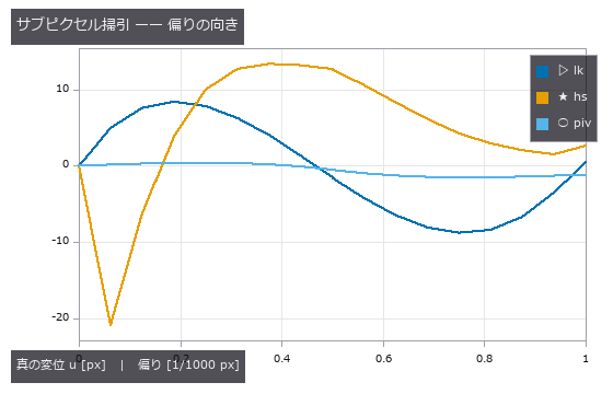
↑ lk は 0.5 px 側へ寄る(教科書の peak locking と逆)。
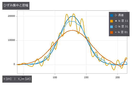
↑ 窓を広げると尖頭が下がり幅が広がる(空間分解能の限界)。
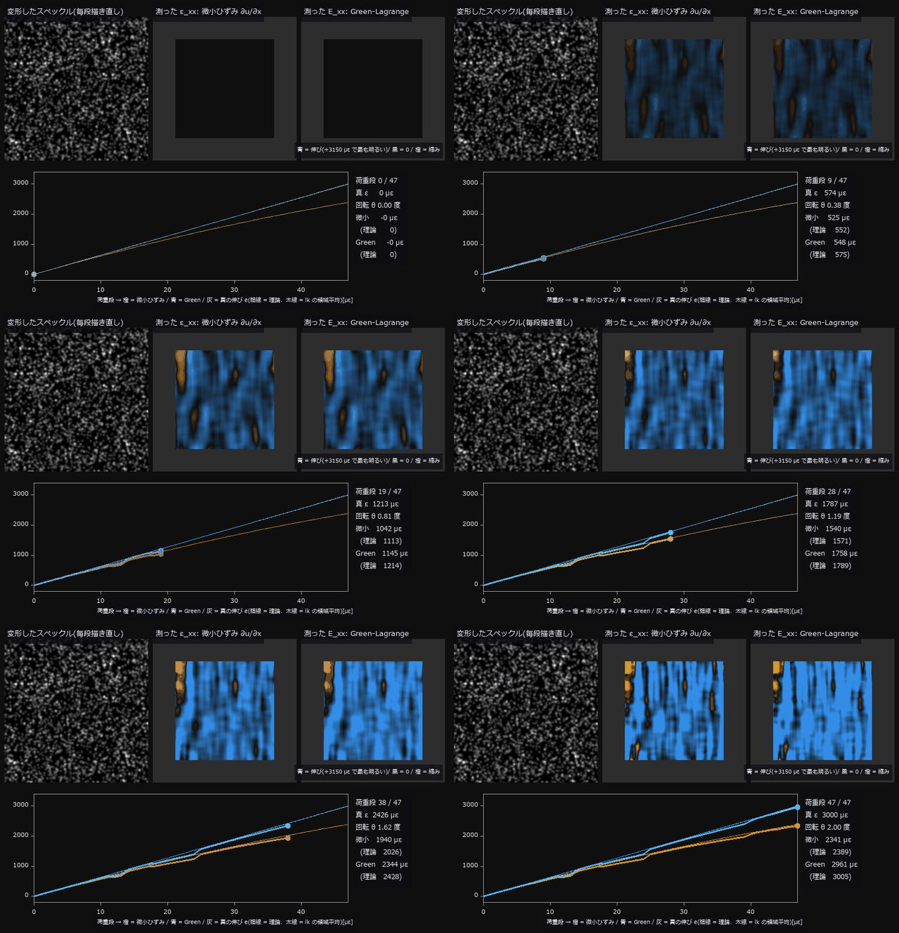
↑ The animation ―― 引張試験の荷重を 48 段で上げる過程(lk、窓 31)。真のひずみを 0 → 3000 µε、同時に試験機が 0 → 2.0 度回る。変形像は毎段、斑点を写して描き直す(補間なし)。最終段で微小ひずみ ∂u/∂x の領域平均は 2341 µε(理論 (1+e)cosθ-1 = 2389 µε)—— 材料は 3000 µε 伸びているのに、回転が約 611 µε 少なく見せる。Green-Lagrange は 2961 µε(理論 e+e²/2 = 3005 µε)。地図の色は全コマ共通の尺度。
py -3.11 examples/poc_dic_strain.py
Source: examples/poc_dic_strain.py
This run produced 5 figures in total - see them all
Ops used (notes): axes_frame · axes_transform · piv_cross_correlate · plot_series · strain_from_displacement · text_box · ticks
No.2026.097 —— Die tilt and TSV overlay from one CT — tilt fakes rotation too
Two stacked dies carry a 7x7 TSV lattice with a planted overlay of (+0.800, -0.450) um, +0.01500 deg of rotation and a die tilt of (1.20, 0.70) deg; a single CT volume is the whole measurement. Comparing the top-surface via openings directly misses by 2.419 um — 2.4x the +-1.0 um spec, and larger than the 0.918 um real overlay. The bias matches the closed form ‘die thickness x lateral part of the top-surface normal’ to a ratio of 0.996 / 0.999, and re-projecting each via down its own fitted axis recovers the truth to 0.0023 um. The prediction that failed: tilt fakes rotation as well as translation, through the sin(alpha)sin(beta) shear of Rx Ry — predicted +0.00733 deg against +0.00696 deg measured as the difference from the zero-tilt control. Axis correction does not remove it; only de-projecting with the measured tilt does. The cliff lands at 0.492 deg measured against 0.491 deg predicted.
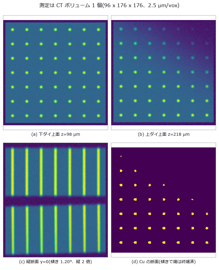
↑ Die tilt and TSV overlay from one CT — tilt fakes rotation too ―― Two stacked dies carry a 7x7 TSV lattice with a planted overlay of (+0.800, -0.450) um, +0.01500 deg of rotation and a die tilt of (1.20, 0.70) deg; a single CT volume is the whole measurement. Comparing the top-surface via openings directly misses by 2.419 um — 2.4x the +-1.0 um spec, and larger than the 0.918 um real overlay. The bias matches the closed form ‘die thickness x lateral part of the top-surface normal’ to a ratio of 0.996 / 0.999, and re-projecting each via down its own fitted axis recovers the truth to 0.0023 um. The prediction that failed: tilt fakes rotation as well as translation, through the sin(alpha)sin(beta) shear of Rx Ry — predicted +0.00733 deg against +0.00696 deg measured as the difference from the zero-tilt control. Axis correction does not remove it; only de-projecting with the measured tilt does. The cliff lands at 0.492 deg measured against 0.491 deg predicted.

↑ The measurement ―― 雲ごと 2.42 µm ずれるのが傾きの偽装。散らばりの広がりは測定精度。 (figure labels are in Japanese; the numbers are the same)

↑ 偽の回転の予測 +0.00733°、倍率の予測 -147.0 ppm(対照群との差で実測 +0.00696° / -144.5 ppm)。
| [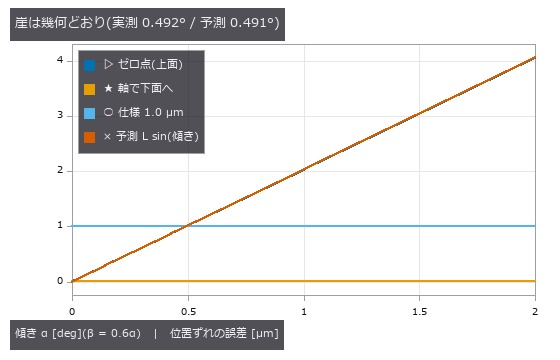](https://raw.githubusercontent.com/furuse-kazufumi/fullseye/master/docs/articles/assets/poc/poc_die_tilt_tsv_overlay/04_tilt_cliff.png) |
| *↑ ゼロ点(青)と予測(赤)は重なっている —— 誤差はダイ厚 x | 法線の横成分 | そのもの。* |

↑ 真の回転 0.01500° を超えるのは α ≈ 1.2°。
py -3.11 examples/poc_die_tilt_tsv_overlay.py
Source: examples/poc_die_tilt_tsv_overlay.py
This run produced 5 figures in total - see them all
Ops used (notes): fit_line3 · procrustes_fit · vol_label
No.2026.014 —— Dimensional Inspection of a Machined Part — Bias and Scatter as Two Numbers
A part defined by a signed distance function (slot width 50.50 px, 1 px = 12.5 µm), imaged through a known PSF (point spread function) and noise and measured by four caliper systems. Otsu’s integer width (the null) has an RMS error of 0.464 px = 5.8 µm; the buried 1-D measuring implementation is biased by -0.0113 px = -0.14 µm, 41x better. Once the edge spacing drops below 3.09 PSF widths the width comes out systematically large, and the API keeps returning success.
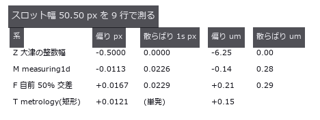
↑ Dimensional Inspection of a Machined Part — Bias and Scatter as Two Numbers ―― A part defined by a signed distance function (slot width 50.50 px, 1 px = 12.5 µm), imaged through a known PSF (point spread function) and noise and measured by four caliper systems. Otsu’s integer width (the null) has an RMS error of 0.464 px = 5.8 µm; the buried 1-D measuring implementation is biased by -0.0113 px = -0.14 µm, 41x better. Once the edge spacing drops below 3.09 PSF widths the width comes out systematically large, and the API keeps returning success.
Terms: PSF — The spatial response of an imaging system to a point object, describing how that point is blurred in the image.; Otsu — A histogram thresholding method that chooses the threshold maximizing the variance between the two resulting classes.
| [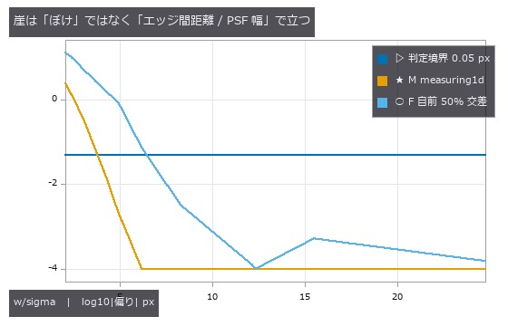](https://raw.githubusercontent.com/furuse-kazufumi/fullseye/master/docs/articles/assets/poc/poc_dimensional_inspection/02_blur_cliff.png) |
| *↑ The measurement ―― 偏りはどちらも正(対が互いを押し広げる)。符号が一定なので繰り返し測っても消えない。下端 -4 は表示の打ち切り( | 偏り | < 1e-4 px)。 (figure labels are in Japanese; the numbers are the same)* |
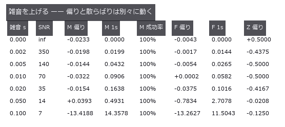
↑ 偏りは SNR 140 まで動かず、増えるのは散らばりだけ。
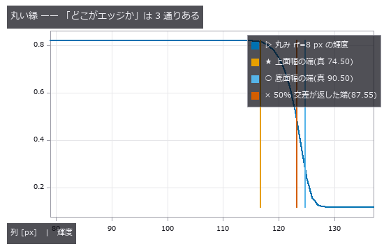
↑ 3 本の縦線は 16.0 px = 200 um 離れている。
py -3.11 examples/poc_dimensional_inspection.py
Source: examples/poc_dimensional_inspection.py
This run produced 4 figures in total - see them all
Ops used (notes): add_metrology_object_circle_measure · add_metrology_object_ellipse_measure · add_metrology_object_generic · add_metrology_object_line_measure · add_metrology_object_rectangle2_measure · align_metrology_model · apply_metrology_model · create_metrology_model · edge_points · ellipse · fuzzy_measure_pairing · gen_measure_arc · gen_measure_rectangle2 · m1_measure_pairs · m1_measure_pos · measure_pairs · measure_pos · otsu · translate_measure
No.2026.018 —— Fibre Orientation Distribution — Angles Repeat Every 180 Degrees, and a Naive Mean Is 90 Degrees Off
Orientation of 140 fibres drawn from a von Mises distribution, read with a structure tensor. For a true mean of 177.9 degrees the arithmetic mean reports 105.55 degrees (-72.33), while the doubled-angle circular mean is off by +0.17 degrees — with not one bit of the image or the measurement changed. Weighting every pixel equally drops the orientation index by -31.3 %.
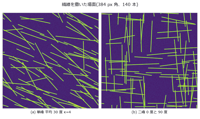
↑ Fibre Orientation Distribution — Angles Repeat Every 180 Degrees, and a Naive Mean Is 90 Degrees Off ―― Orientation of 140 fibres drawn from a von Mises distribution, read with a structure tensor. For a true mean of 177.9 degrees the arithmetic mean reports 105.55 degrees (-72.33), while the doubled-angle circular mean is off by +0.17 degrees — with not one bit of the image or the measurement changed. Weighting every pixel equally drops the orientation index by -31.3 %.
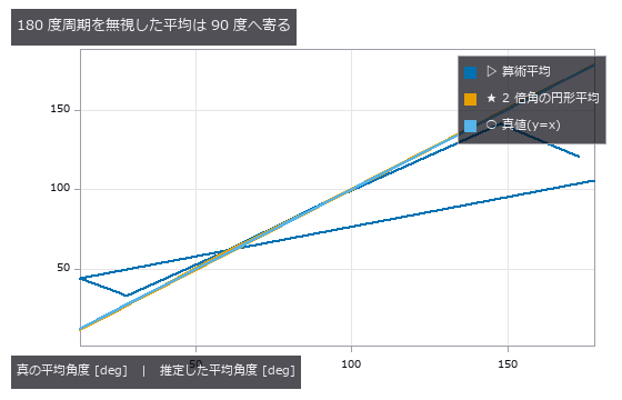
↑ The measurement (figure labels are in Japanese; the numbers are the same)
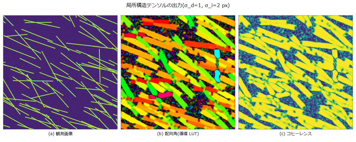
↑ この回の図
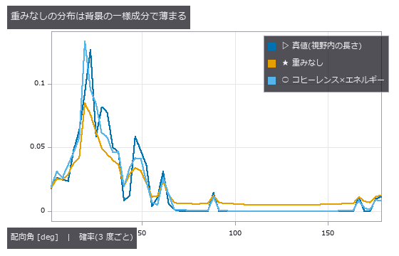
↑ この回の図
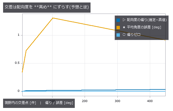
↑ この回の図
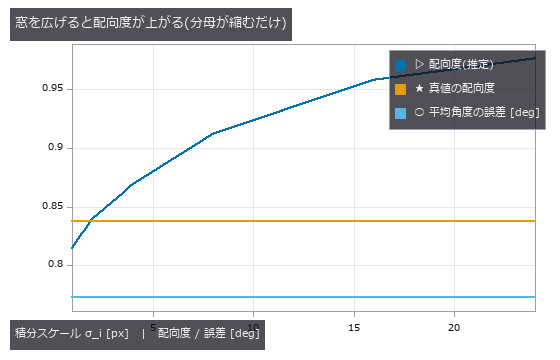
↑ この回の図
py -3.11 examples/poc_fiber_orientation.py
Source: examples/poc_fiber_orientation.py
This run produced 6 figures in total - see them all
Ops used (notes): coherence · dc_structure_texture · moment_axes · principal_moments · smooth_funct_1d_gauss · sobel_amp · sobel_dir
No.2026.021 —— Gear Tooth Metrology — Eccentricity Is Order 1, Teeth Are Order z
Eccentricity and tooth profile read from a gear drawn with the closed-form involute. The null’s least-squares circle has a diameter of 47.278 mm, which is neither the pitch (48), tip (52) nor root (43) circle. One missing tooth turns an eccentricity of 0.050 mm into 0.1285 mm (+157 %); the traditional method of one sample per tooth returns 0.0501 mm (+0.2 %).
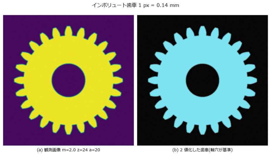
↑ Gear Tooth Metrology — Eccentricity Is Order 1, Teeth Are Order z ―― Eccentricity and tooth profile read from a gear drawn with the closed-form involute. The null’s least-squares circle has a diameter of 47.278 mm, which is neither the pitch (48), tip (52) nor root (43) circle. One missing tooth turns an eccentricity of 0.050 mm into 0.1285 mm (+157 %); the traditional method of one sample per tooth returns 0.0501 mm (+0.2 %).
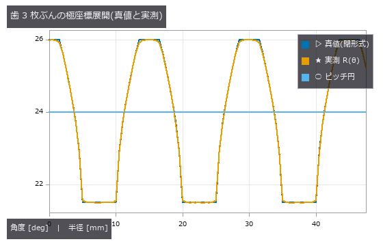
↑ The measurement (figure labels are in Japanese; the numbers are the same)
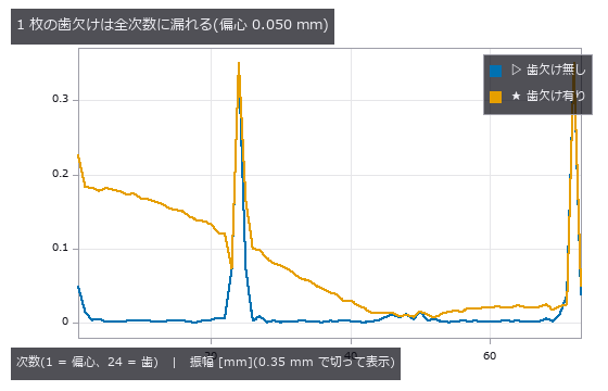
↑ 歯の次数 24/48/72 は 2.6 mm あるので 0.35 mm で切った
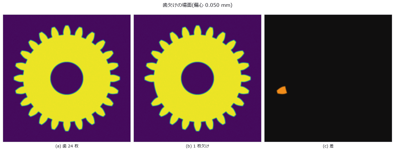
↑ この回の図
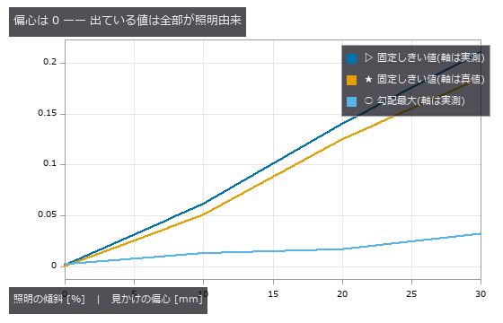
↑ この回の図
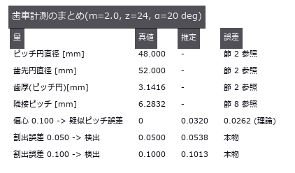
↑ この回の図
py -3.11 examples/poc_gear_tooth_metrology.py
Source: examples/poc_gear_tooth_metrology.py
This run produced 6 figures in total - see them all
Ops used (notes): blob_boundaries · blob_features · blob_label · blob_overlay · blob_region · blob_select_largest · gauss_filter · polar_trans_image · spectrum · threshold
No.2026.073 —— Metallographic Grain Size — The Planimetric and Intercept Methods Fall Off Different Cliffs
Grains are synthesized as a 2-D Voronoi tessellation with 2-px boundaries, then etching unevenness, noise and boundary gaps are added; ASTM E112 grain size G is measured by the planimetric method (Otsu + connected components) and the lineal-intercept method (local threshold + test lines in 4 directions). The planimetric method survives noise alone (-0.02) and etching unevenness alone (-0.40) but dies under both (+3.82), and loses one G step at 7.2 % boundary gaps; the intercept method holds to 40.7 % — the predicted 29.3 % was wrong because only 0.76 f of the boundary actually disappears in the mask. A duplex structure gives a whole-field G of 7.82 that matches neither the fine (9.01) nor the coarse (6.15) population; only 4 of 64 tiles fall within ±0.5 of it.

↑ Metallographic Grain Size — The Planimetric and Intercept Methods Fall Off Different Cliffs ―― Grains are synthesized as a 2-D Voronoi tessellation with 2-px boundaries, then etching unevenness, noise and boundary gaps are added; ASTM E112 grain size G is measured by the planimetric method (Otsu + connected components) and the lineal-intercept method (local threshold + test lines in 4 directions). The planimetric method survives noise alone (-0.02) and etching unevenness alone (-0.40) but dies under both (+3.82), and loses one G step at 7.2 % boundary gaps; the intercept method holds to 40.7 % — the predicted 29.3 % was wrong because only 0.76 f of the boundary actually disappears in the mask. A duplex structure gives a whole-field G of 7.82 that matches neither the fine (9.01) nor the coarse (6.15) population; only 4 of 64 tiles fall within ±0.5 of it.
Terms: Otsu — A histogram thresholding method that chooses the threshold maximizing the variance between the two resulting classes.

↑ The measurement (figure labels are in Japanese; the numbers are the same)

↑ この回の図

↑ 面積法は 1 本の途切れで 2 粒が融合するので、切片法の 6 分の 1 の途切れで 1 段落ちる。

↑ この回の図

↑ この回の図
py -3.11 examples/poc_metal_grain_size.py
Source: examples/poc_metal_grain_size.py
This run produced 11 figures in total - see them all
Ops used (notes): bin_threshold · blob_features · blob_label · blob_overlay · bothat · dyn_threshold · gray_bothat · hx_close_edges · invert_image · otsu · threshold
No.2026.100 —— Why the Seafloor Smiles — Sound-Speed Error Remaining on Outer Beams After Nadir Calibration
In multibeam echosounding, a wrong sound-speed profile bends a flat bottom. Using surface sound speed directly also shifts nadir by +0.670 m; after calibrating mean sound speed at nadir, nadir error is zero but −2.697 m remains at 65 degrees. IHO S-44 Order 1a TVU at 50 m is 0.8201 m. The pre-fix TVU breach attributed to layer spacing was actually an omitted first-layer Snell conversion; after preserving the ray parameter from the first layer, the midpoint iso-velocity approximation is −0.016 m with two layers at 65 degrees, converges at about second order, and is within TVU. In this synthetic model amplitude-peak bias grows on outer beams, consistent with an advantage of phase detection, but it does not establish the design history of real instruments. The truth-free check implemented here is overlap comparison between adjacent lines (2.697 m at the edge). Under upward refraction, beams beyond the critical angle disappear while the reachable 65-degree beam still has +5.919 m depth error. A constant-gradient fit reduces the maximum error by 77%, from 5.357 m to 1.253 m, but leaves a TVU-breaching residual and worsens nadir by +0.262 m.
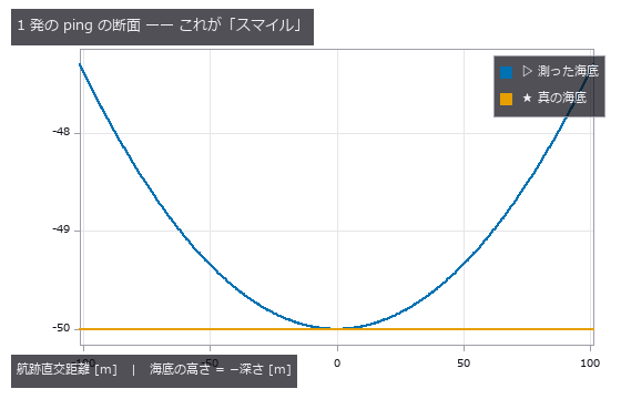
↑ Why the Seafloor Smiles — Sound-Speed Error Remaining on Outer Beams After Nadir Calibration ―― In multibeam echosounding, a wrong sound-speed profile bends a flat bottom. Using surface sound speed directly also shifts nadir by +0.670 m; after calibrating mean sound speed at nadir, nadir error is zero but −2.697 m remains at 65 degrees. IHO S-44 Order 1a TVU at 50 m is 0.8201 m. The pre-fix TVU breach attributed to layer spacing was actually an omitted first-layer Snell conversion; after preserving the ray parameter from the first layer, the midpoint iso-velocity approximation is −0.016 m with two layers at 65 degrees, converges at about second order, and is within TVU. In this synthetic model amplitude-peak bias grows on outer beams, consistent with an advantage of phase detection, but it does not establish the design history of real instruments. The truth-free check implemented here is overlap comparison between adjacent lines (2.697 m at the edge). Under upward refraction, beams beyond the critical angle disappear while the reachable 65-degree beam still has +5.919 m depth error. A constant-gradient fit reduces the maximum error by 77%, from 5.357 m to 1.253 m, but leaves a TVU-breaching residual and worsens nadir by +0.262 m.
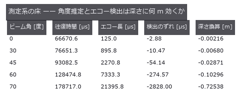
↑ The measurement ―― エコーは beamform_delay_sum の角度応答 × Lambert 後方散乱で海底の帯を足し上げて合成。find_peaks + peak_subbin で検出。 (figure labels are in Japanese; the numbers are the same)
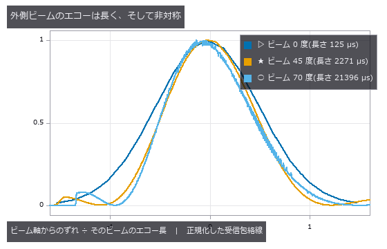
↑ 長さは 125 / 2271 / 21396 µs(170 倍の開き)。
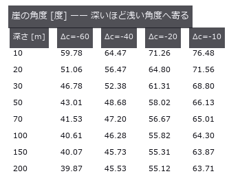
↑ Δc = -40 m/s の深水漸近値は 44.83 度。
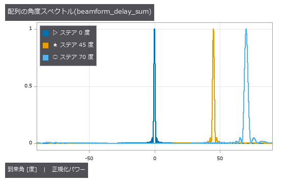
↑ 素子 96 本・λ/2 間隔。
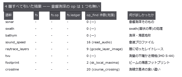
↑ ○ = 在る。
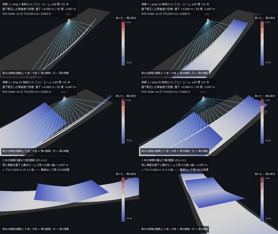
↑ The animation ―― 主図(動画、640 × 360・30 fps・12 秒): 深さ 50 m の平らな海底を、船が 2 本の測線(間隔 101.4 m)で測る。水色は真の音線(水柱の音速差 -40 m/s の線形プロファイルで円弧に曲がる)、白い点と面は直下較正した等音速の処理が記録する海底で、色は「測った − 真の深さ」(高さの誤差だけ画面上 5 倍)。直下は +0.000 m、65 度は -2.697 m —— 平らな海底が外側だけ持ち上がる「スマイル」。最後に重なり帯を回り込むと、同じ海底を直下と最外ビームで測った 2.697 m の段差(TVU 0.820 m の 3.3 倍)が立っている。
py -3.11 examples/poc_multibeam_bathymetry.py
Source: examples/poc_multibeam_bathymetry.py
This run produced 19 figures in total - see them all
Ops used (notes): beamform_delay_sum · beamform_doa · color_bar · dem_slope · find_peaks · intensity · interp_scattered · peak_subbin · snell_angle · text_box
No.2026.029 —— Particle Size Distribution From Images — Merging and Edge Cuts Pull Opposite Ways and Cancel
D10 / D50 / D90 from a synthetic scatter of particles, with merges (pulling large) and edge cuts (pulling small) counted separately. At an area fraction of 13.8 % the D50 error is +0.55 % — because 28 merges and 19 edge cuts happen to balance. Number- and area-weighting give D50 values of 26.9 and 44.7 µm (1.66x) from the same blobs.
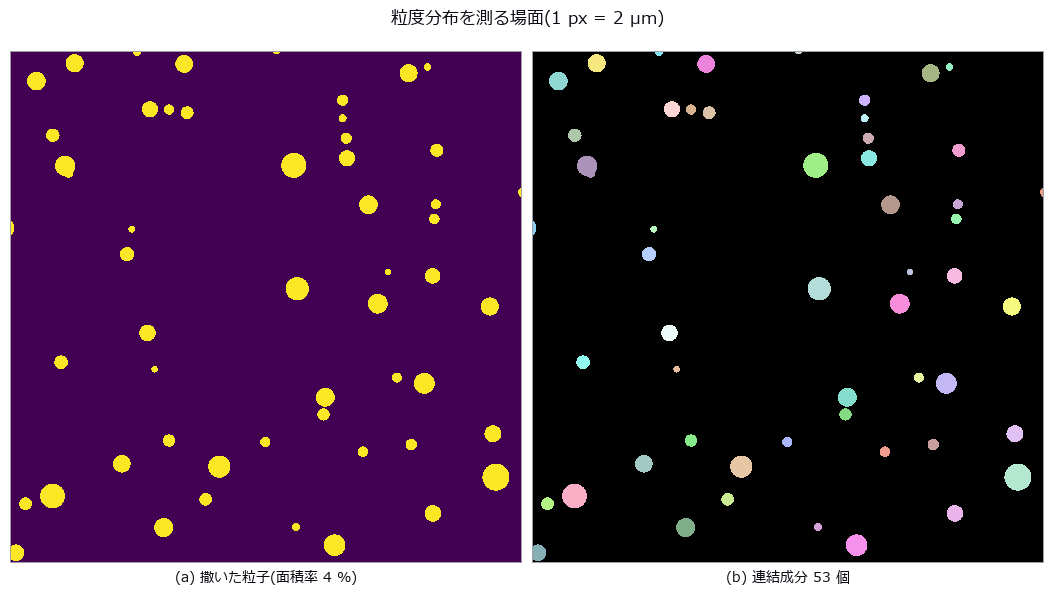
↑ Particle Size Distribution From Images — Merging and Edge Cuts Pull Opposite Ways and Cancel ―― D10 / D50 / D90 from a synthetic scatter of particles, with merges (pulling large) and edge cuts (pulling small) counted separately. At an area fraction of 13.8 % the D50 error is +0.55 % — because 28 merges and 19 edge cuts happen to balance. Number- and area-weighting give D50 values of 26.9 and 44.7 µm (1.66x) from the same blobs.
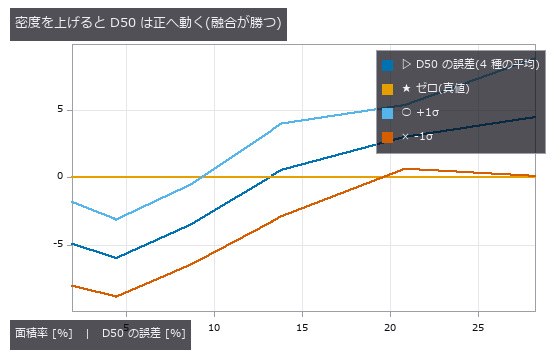
↑ The measurement ―― 薄いところで 0 なのは正確だから。濃いところで 0 をまたぐのは融合と縁切れが釣り合っただけ。 (figure labels are in Japanese; the numbers are the same)
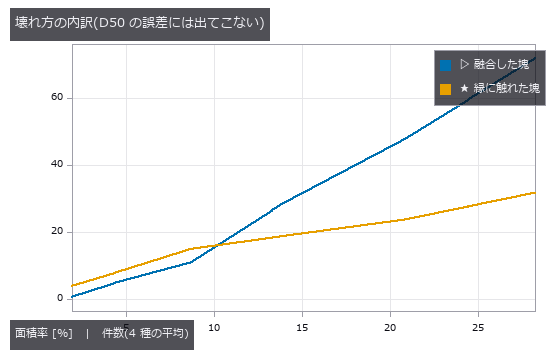
↑ この回の図
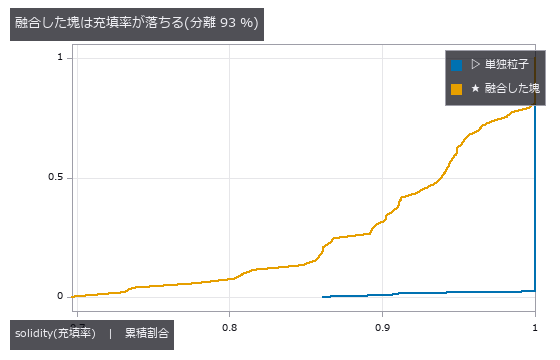
↑ この回の図

↑ この回の図
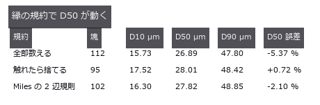
↑ この回の図
py -3.11 examples/poc_particle_sizing.py
Source: examples/poc_particle_sizing.py
This run produced 7 figures in total - see them all
Ops used (notes): blob_features · blob_label · blob_overlay · blob_region · blob_select · circularity · distance_transform
No.2026.031 —— Stress by Photoelasticity — Unwrapping Fails First at the Isotropic Point
Viewed through polarisers, a loaded transparent plastic shows its internal stress as fringes. Stress in a squeezed disc was recovered from polarisation images, including pixels where the fringe order exceeds 0.5 and the phase wraps. Recovery fails first at isotropic points where fringe contrast drops.
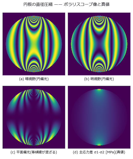
↑ Stress by Photoelasticity — Unwrapping Fails First at the Isotropic Point ―― The closed-form stress field of a diametrally loaded disc (4.2441 MPa at the centre, fringe order 2.380) turned into polariscope images by the Mueller-matrix (4-by-4 polarization-transfer matrix) ops and read back to stress. The op-built polariscope matches the textbook formula to 2.2e-16 across 125 cases. Phase wraps in the 84.2 % of pixels above fringe order 0.5, and unwrapping breaks first not where stress is highest but at the isotropic point, where modulation vanishes.
Terms: Mueller matrix — A real 4-by-4 matrix acting on a Stokes vector to describe how an optical element or sample changes polarization.
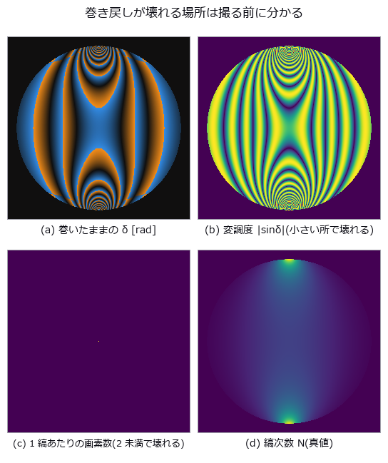
↑ The measurement ―― 左下 2 枚が「壊れる予報」。予報は当たるが、外せば直るとは限らない。 (figure labels are in Japanese; the numbers are the same)
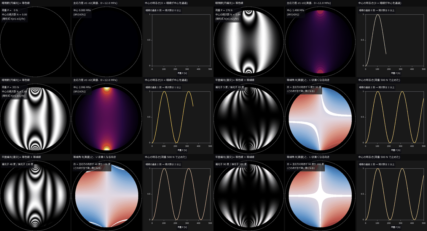
↑ The animation ―― 動画(230 コマ、円板 φ50 mm を 361 画素で描画、半径 0.9R の外は描かない): 前半は荷重を 0 → 500 N へ上げる。暗視野(円偏光)の暗線は縞次数が整数の等値線で、荷重点から湧き出して中心へ寄る。中心の縞次数は荷重に比例して 2.38 まで増え(閉形式 h(σ1-σ2)/fσ)、右のグラフの中心の明るさ sin²(πN) が 0 に落ちるたびに暗線が中心を通過する(通過 2 回)。後半は荷重 500 N のまま、直交させた平面偏光子の対を 0 → 90 度回す。平面偏光の黒には 2 種類あり、回しても動かない縞は等色線(暗視野と同じ)、回すと動く黒い帯が等傾線 = 主応力の向きが偏光子と平行か直交する点で、中央の真値 θ の図で白く塗った点と重なる。偏光系は fullseye の mueller_element / mueller_apply(暗視野)と sin²(2(θ-β))·sin²(δ/2)(平面)。
py -3.11 examples/poc_photoelasticity.py
Source: examples/poc_photoelasticity.py
This run produced 3 figures in total - see them all
Ops used (notes): axes_frame · axes_transform · mueller_apply · mueller_element · plot_series · text_box · ticks · unwrap_phase_2d
No.2026.103 —— Measuring Rail with a Chord — At the Wavelengths Where the Transfer Function Is Zero, Any Amplitude Reads Zero
| Reading track irregularity with a chord (versine) — the distance from the mid-point to a chord drawn between two points, still the working method in track recording and in acceptance of rail re-profiling. The null baseline, reading the versine directly as height, ranges from 0.0 % to 200.0 % of the truth depending on wavelength: one and the same 10 m chord reads lambda=10 m at +100 %, lambda=1.5 m at +50 %, lambda=30 m at -50 %, and lambda=5.0 / 2.5 / 1.0 m at -100 %. Over-reading and under-reading happen at once, so no single correction factor repairs it. The blind spots are exact geometry: | H(lambda) | = | 1 - cos(pi L / lambda) | is exactly zero at lambda = L/(2n) and doubles at lambda = L/(2n+1). Across ten wavelengths and two chords, twenty cases, prediction and measurement differ by at most 0.00000, and a 0.600 mm undulation at lambda=5.00 m gives a versine whose largest absolute value over 200 m is 0.00000 mm. Sorting into third-octave wavelength bands does not remove it (the ratio spans 0.00041 to 2.000, a factor of 4924), and the operator’s total_power earned its place here: the band sum is only 0.519 of the sum over all FFT bins, and the missing 48 % is the 30 m irregularity sitting below f_min — invisible if only the bands are read. Dividing by | H | to invert diverges to 6.9e7 mm at the blind wavelengths, and regularising it makes three wavelengths quietly report ‘no irregularity’. Two chords (10 m and 6 m) recover eight of the ten wavelengths to within 0.1 %, but the shared blind spot is not a point: it is the comb lambda = 1.000/k. One prediction was wrong — the planted lambda=0.100 m also survived, and it turned out to be the k=10 tooth. The relative spacing of the comb equals lambda itself, so it thickens toward short wavelengths: the corrugation band 0.03-0.30 m alone holds 30 blind wavelengths. At the 0.25 m sampling of a recording car, a 30 mm corrugation reappears as a 0.750 m undulation of 0.0528 mm, nine times the 0.00584 mm floor of a control with the short waves switched off. An asymmetric chord (3.7 m and 6.3 m arms) removes the long-wave blind spots, but | H | = 0 requires a/lambda and b/lambda to be integers together, so the blind spots move to lambda = gcd(a, b)/k = 0.100 m: the chord built to measure corrugation is blind inside the corrugation band. |

| *↑ Measuring Rail with a Chord — At the Wavelengths Where the Transfer Function Is Zero, Any Amplitude Reads Zero ―― Reading track irregularity with a chord (versine) — the distance from the mid-point to a chord drawn between two points, still the working method in track recording and in acceptance of rail re-profiling. The null baseline, reading the versine directly as height, ranges from 0.0 % to 200.0 % of the truth depending on wavelength: one and the same 10 m chord reads lambda=10 m at +100 %, lambda=1.5 m at +50 %, lambda=30 m at -50 %, and lambda=5.0 / 2.5 / 1.0 m at -100 %. Over-reading and under-reading happen at once, so no single correction factor repairs it. The blind spots are exact geometry: | H(lambda) | = | 1 - cos(pi L / lambda) | is exactly zero at lambda = L/(2n) and doubles at lambda = L/(2n+1). Across ten wavelengths and two chords, twenty cases, prediction and measurement differ by at most 0.00000, and a 0.600 mm undulation at lambda=5.00 m gives a versine whose largest absolute value over 200 m is 0.00000 mm. Sorting into third-octave wavelength bands does not remove it (the ratio spans 0.00041 to 2.000, a factor of 4924), and the operator’s total_power earned its place here: the band sum is only 0.519 of the sum over all FFT bins, and the missing 48 % is the 30 m irregularity sitting below f_min — invisible if only the bands are read. Dividing by | H | to invert diverges to 6.9e7 mm at the blind wavelengths, and regularising it makes three wavelengths quietly report ‘no irregularity’. Two chords (10 m and 6 m) recover eight of the ten wavelengths to within 0.1 %, but the shared blind spot is not a point: it is the comb lambda = 1.000/k. One prediction was wrong — the planted lambda=0.100 m also survived, and it turned out to be the k=10 tooth. The relative spacing of the comb equals lambda itself, so it thickens toward short wavelengths: the corrugation band 0.03-0.30 m alone holds 30 blind wavelengths. At the 0.25 m sampling of a recording car, a 30 mm corrugation reappears as a 0.750 m undulation of 0.0528 mm, nine times the 0.00584 mm floor of a control with the short waves switched off. An asymmetric chord (3.7 m and 6.3 m arms) removes the long-wave blind spots, but | H | = 0 requires a/lambda and b/lambda to be integers together, so the blind spots move to lambda = gcd(a, b)/k = 0.100 m: the chord built to measure corrugation is blind inside the corrugation band.* |

↑ The measurement (figure labels are in Japanese; the numbers are the same)

↑ 10 m 弦は λ=5.0 / 2.5 / 1.67 / 1.25 / 1.0 m で厳密に 0、λ=10 / 3.33 m で 2 倍。

↑ この回の図

↑ この回の図

↑ 0.750 m の周期がきれいに立つ。
py -3.11 examples/poc_rail_corrugation.py
Source: examples/poc_rail_corrugation.py
This run produced 11 figures in total - see them all
Ops used (notes): octave_bands · octave_spectrum
No.2026.104 —— Counting and Measuring Real Coins — A Correct Answer Is Not a Safe One
The real photograph famous for ‘a global threshold cannot work here, the lighting falls away across the frame’ (scikit-image coins). The background does slope, 0.427 to 0.161 down the rows and 0.331 to 0.059 across the columns — and yet a plain global Otsu with hole filling and an area floor of 150 lands exactly on the true 24. The truth is fixed by three independent paths agreeing (an area plateau spanning 50 to 800, a Hough circle search with the radii stated explicitly, and Sobel plus hole filling) and then checked one-to-one, each circle falling inside exactly one component. The margin, however, is 0.05: adding a little more of the same slope drops the count to 22. A correct answer is not evidence of a safe one. At +0.30 the median area moves by only -0.33 % while the worst single coin moves -27.26 %, and the drift correlates with row position at r = -0.91 — true area does not depend on where a coin sits, so that correlation is error, entire. Flattening with gray_tophat keeps the count but shrinks the median area to 0.29x, and the raw component count differs by 30 % between 4- and 8-connectivity.
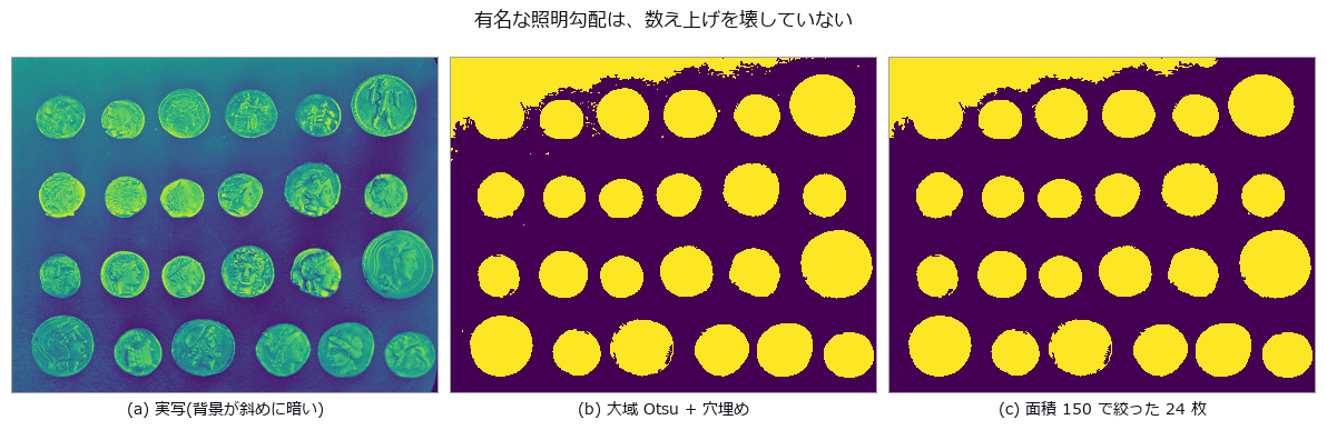
↑ Counting and Measuring Real Coins — A Correct Answer Is Not a Safe One ―― The real photograph famous for ‘a global threshold cannot work here, the lighting falls away across the frame’ (scikit-image coins). The background does slope, 0.427 to 0.161 down the rows and 0.331 to 0.059 across the columns — and yet a plain global Otsu with hole filling and an area floor of 150 lands exactly on the true 24. The truth is fixed by three independent paths agreeing (an area plateau spanning 50 to 800, a Hough circle search with the radii stated explicitly, and Sobel plus hole filling) and then checked one-to-one, each circle falling inside exactly one component. The margin, however, is 0.05: adding a little more of the same slope drops the count to 22. A correct answer is not evidence of a safe one. At +0.30 the median area moves by only -0.33 % while the worst single coin moves -27.26 %, and the drift correlates with row position at r = -0.91 — true area does not depend on where a coin sits, so that correlation is error, entire. Flattening with gray_tophat keeps the count but shrinks the median area to 0.29x, and the raw component count differs by 30 % between 4- and 8-connectivity.
Terms: Otsu — A histogram thresholding method that chooses the threshold maximizing the variance between the two resulting classes.
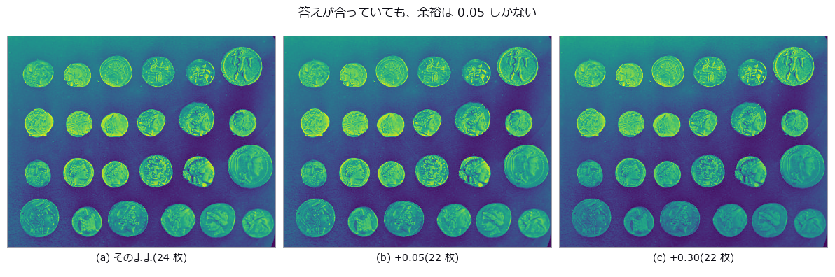
↑ The measurement ―― 見た目はほとんど変わらないのに 2 枚落ちる。 (figure labels are in Japanese; the numbers are the same)
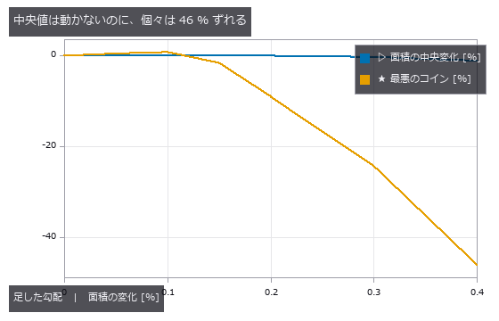
↑ 代表値で報告すると、壊れているのに壊れていないように見える。
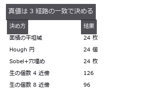
↑ 生の個数は近傍の規約で 3 割違う。
py -3.11 examples/poc_real_coin_metrology.py
Source: examples/poc_real_coin_metrology.py
This run produced 4 figures in total - see them all
Ops used (notes): blob_count · blob_features · blob_label · canny · fill_holes · gray_tophat · hough_circle_trans · otsu · sobel_amp
No.2026.083 —— Pitch, Flank Angle and Pitch Diameter From a Thread Silhouette — Tilt Shows Up With Opposite Signs on the Two Flanks
An M6-like silhouette drawn from the ISO 68-1 basic triangle in closed form (1 px = 25 µm). An FFT of the binarised column widths reports half the true pitch, 20 px, because the two profiles are offset by P/2 and their sum is constant. Tilting the axis by 3 degrees splits the flank angles into 33.18 / 26.74 degrees: their half-sum 29.81 is the true flank angle and their half-difference 3.19 estimates the tilt. Pitch measured on one flank drifts at first order (+3.28 / -2.79 %) while the crest spacing drifts at second order (-0.12 %); undoing the tilt leaves P -0.009 % and d2 +0.033 %.
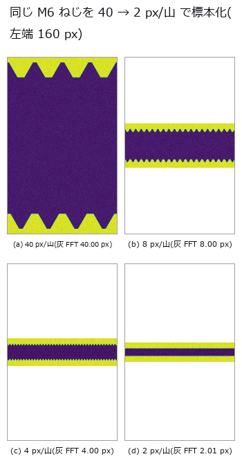
↑ Pitch, Flank Angle and Pitch Diameter From a Thread Silhouette — Tilt Shows Up With Opposite Signs on the Two Flanks ―― An M6-like silhouette drawn from the ISO 68-1 basic triangle in closed form (1 px = 25 µm). An FFT of the binarised column widths reports half the true pitch, 20 px, because the two profiles are offset by P/2 and their sum is constant. Tilting the axis by 3 degrees splits the flank angles into 33.18 / 26.74 degrees: their half-sum 29.81 is the true flank angle and their half-difference 3.19 estimates the tilt. Pitch measured on one flank drifts at first order (+3.28 / -2.79 %) while the crest spacing drifts at second order (-0.12 %); undoing the tilt leaves P -0.009 % and d2 +0.033 %.
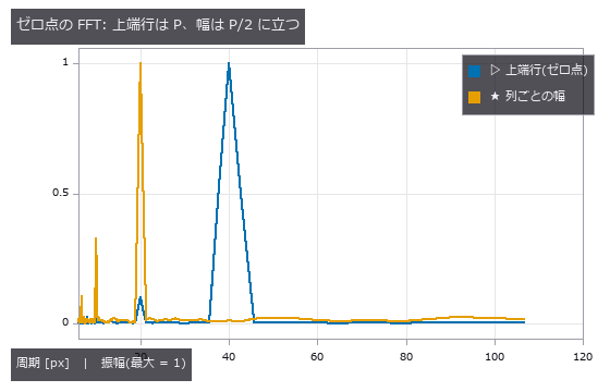
↑ The measurement ―― 幅の系列は上下輪郭(P/2 ずれ)の和なので基本波が消える。 (figure labels are in Japanese; the numbers are the same)
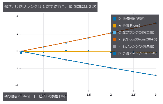
↑ 片側のフランクだけで測ると 1 度あたり約 1 % 狂う。
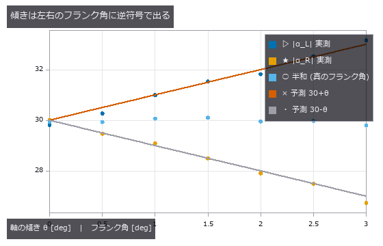
↑ 半差が θ、半和が α。

↑ 生 = 水平 caliper 4 山、補正 = θ_est の向きの caliper 16 山(3 種の平均)。
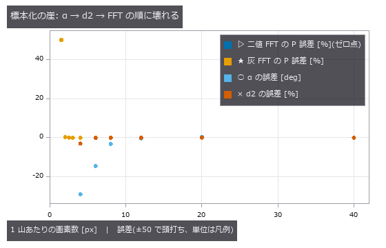
↑ 測れなかった点は描かない。
py -3.11 examples/poc_screw_thread_metrology.py
Source: examples/poc_screw_thread_metrology.py
This run produced 9 figures in total - see them all
Ops used (notes): fit_line_contours · gen_measure_rectangle2 · hx_split_contours · measure_pos · threshold · threshold_sub_pix · xg_regress_contours
No.2026.112 —— Stockpile Inventory — The Answer Is Fixed by the Ground Nobody Measured
Stockpile inventory from a 3-D scan, for mining, aggregates and ports. The pile and the ground beneath it are written as separate formulas, and making the pile a sum of three cones at a 37 degree angle of repose closes the volume analytically at 3572.6089 m^3, matching a numerical integration at 0.025 m cells. The point is that the single number everyone quotes is fixed by a surface nobody measured: the ground under the pile. The first cliff is the assumed base, stated in closed form as dV = -A dh before measuring and matching to 0.0000 m^3 over seven offsets. The surprise is not the agreement but the size: 5 cm, which no survey would call an error, is 1.269 % of the inventory, or 72.5 t at a bulk density of 1.6 t/m^3 — three truckloads. The second cliff is occlusion. A cone is a ruled surface, so the visible fraction is arccos((H - h_s)/(D tan phi))/pi, matching to within 0.0201 over six geometries, and that residual halves with the cell size (0.0339, 0.0171, 0.0120 at 1.2, 0.6 and 0.4 m), which identifies it as discretisation rather than a wrong model. One prediction was wrong: interpolating across the occluded side was expected to under-estimate the volume, since a cone is concave and a chord passes below it, but the measurement is +17.20 %, an over-estimate. The far side is hidden all the way to the toe, so the triangulation connects the ridge not to the pile but to the ground beyond it, and a chord thrown 30 m past the ridge has a slope of 0.37 m/m that passes above the true 0.75 m/m slope. Then a cancellation trap: with the same single scan, using the true ground gives +17.20 % while the field practice of a horizontal base at the mean perimeter height gives +0.51 %. Nothing improved — the perimeter was lifted by the same interpolation, by +0.728 m, and the subtraction hides it; using only the perimeter points that were actually seen returns +12.05 %. A contaminated ruler applied to a contaminated object makes the error look like it went away. The same shape recurs with a berm of spoil at the toe: the outlier-resistant RANSAC fit reads worse (+2.48 %) than total least squares (+0.61 %), but RANSAC correctly rejected the berm and returned to the no-berm answer of +1.91 %, while TLS looked good because the berm’s lift happened to cancel the bias from the undulating ground. Averaging the perimeter cancels the ground’s tilt whenever the footprint is roughly symmetric — the flat control reads +0.01 % — so the remaining +1.79 % is entirely undulation, and fitting a tilted plane makes it worse (+1.91 %): more freedom does not mean less bias. The rulers disagree on the winner, with the horizontal base slightly better on volume and the fitted plane six times better on the centroid (0.07 m against 0.42 m), which is the quantity a loading plan uses. And the two errors do not add: -0.70 % expected against +0.51 % measured, because the occlusion fill moves the perimeter that fixes the base. Finally, a real bug was found and fixed: dem_viewshed reported every cell above the observer’s eye as not visible — the apex of a cone on open flat ground read 0.0, none of the 1541 cells above eye level were visible, and the occluded fraction came out 0.8863 against a closed-form 0.5710. Line-of-sight samples rounded onto the target cell itself, occluding it against its own height; skipping those samples restores 1.0 at the apex and 0.5900 for the occluded fraction. The existing tests missed it because they only checked flat ground and what lies behind a wall, never whether the wall itself is visible.
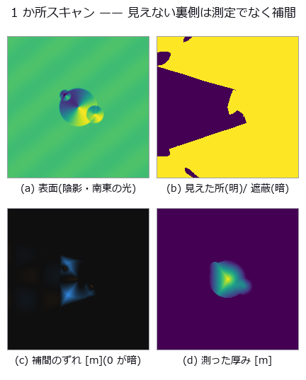
↑ Stockpile Inventory — The Answer Is Fixed by the Ground Nobody Measured ―― Stockpile inventory from a 3-D scan, for mining, aggregates and ports. The pile and the ground beneath it are written as separate formulas, and making the pile a sum of three cones at a 37 degree angle of repose closes the volume analytically at 3572.6089 m^3, matching a numerical integration at 0.025 m cells. The point is that the single number everyone quotes is fixed by a surface nobody measured: the ground under the pile. The first cliff is the assumed base, stated in closed form as dV = -A dh before measuring and matching to 0.0000 m^3 over seven offsets. The surprise is not the agreement but the size: 5 cm, which no survey would call an error, is 1.269 % of the inventory, or 72.5 t at a bulk density of 1.6 t/m^3 — three truckloads. The second cliff is occlusion. A cone is a ruled surface, so the visible fraction is arccos((H - h_s)/(D tan phi))/pi, matching to within 0.0201 over six geometries, and that residual halves with the cell size (0.0339, 0.0171, 0.0120 at 1.2, 0.6 and 0.4 m), which identifies it as discretisation rather than a wrong model. One prediction was wrong: interpolating across the occluded side was expected to under-estimate the volume, since a cone is concave and a chord passes below it, but the measurement is +17.20 %, an over-estimate. The far side is hidden all the way to the toe, so the triangulation connects the ridge not to the pile but to the ground beyond it, and a chord thrown 30 m past the ridge has a slope of 0.37 m/m that passes above the true 0.75 m/m slope. Then a cancellation trap: with the same single scan, using the true ground gives +17.20 % while the field practice of a horizontal base at the mean perimeter height gives +0.51 %. Nothing improved — the perimeter was lifted by the same interpolation, by +0.728 m, and the subtraction hides it; using only the perimeter points that were actually seen returns +12.05 %. A contaminated ruler applied to a contaminated object makes the error look like it went away. The same shape recurs with a berm of spoil at the toe: the outlier-resistant RANSAC fit reads worse (+2.48 %) than total least squares (+0.61 %), but RANSAC correctly rejected the berm and returned to the no-berm answer of +1.91 %, while TLS looked good because the berm’s lift happened to cancel the bias from the undulating ground. Averaging the perimeter cancels the ground’s tilt whenever the footprint is roughly symmetric — the flat control reads +0.01 % — so the remaining +1.79 % is entirely undulation, and fitting a tilted plane makes it worse (+1.91 %): more freedom does not mean less bias. The rulers disagree on the winner, with the horizontal base slightly better on volume and the fitted plane six times better on the centroid (0.07 m against 0.42 m), which is the quantity a loading plan uses. And the two errors do not add: -0.70 % expected against +0.51 % measured, because the occlusion fill moves the perimeter that fixes the base. Finally, a real bug was found and fixed: dem_viewshed reported every cell above the observer’s eye as not visible — the apex of a cone on open flat ground read 0.0, none of the 1541 cells above eye level were visible, and the occluded fraction came out 0.8863 against a closed-form 0.5710. Line-of-sight samples rounded onto the target cell itself, occluding it against its own height; skipping those samples restores 1.0 at the apex and 0.5900 for the occluded fraction. The existing tests missed it because they only checked flat ground and what lies behind a wall, never whether the wall itself is visible.
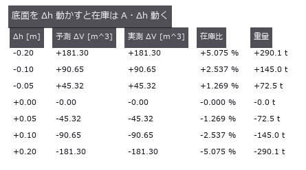
↑ The measurement ―― A = 906.5 m^2。閉形式は測る前に印字してある。 (figure labels are in Japanese; the numbers are the same)
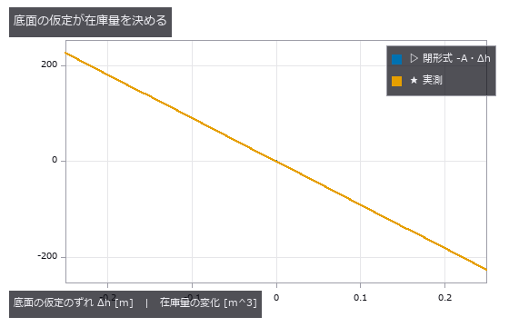
↑ 2 本は重なる。

↑ 可視率 = arccos((H-h_s)/(D tanφ))/π。
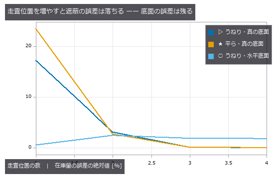
↑ 3 か所で遮蔽は 1.4 % まで落ちるが、うねり由来の +1.8 % は何か所測っても消えない(底面は誰も測っていない)。
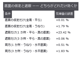
↑ 対照群(平ら/全周)で 2 つを切り分けてから、両方入れる。
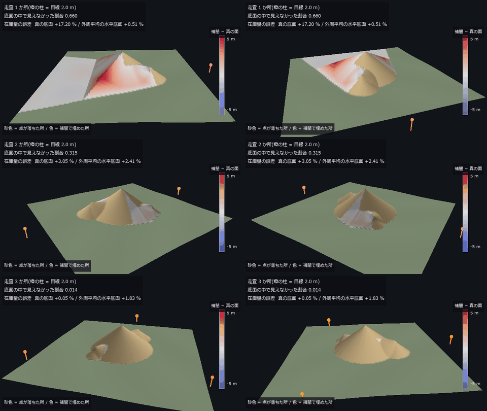
↑ The animation ―― 主図(動画、640 × 360・30 fps・12 秒): うねりのある地面に置いた山の周りを一周しながら、走査位置を 1 → 2 → 3 か所と増やす。描いているのは補間で埋めた DSM(在庫計算が信じている面)で、色は「補間 − 真の面」(最大 5.23 m)。見えなかった割合は 0.660 → 0.315 → 0.014。在庫量の誤差は真の底面で +17.20 % → +3.05 % → +0.05 %、外周平均の水平底面で +0.51 % → +2.41 % → +1.83 % —— 3 か所で遮蔽は塞がるが、うねり由来の偏りは残る。高さは実寸。
py -3.11 examples/poc_stockpile_volume.py
Source: examples/poc_stockpile_volume.py
This run produced 7 figures in total - see them all
Ops used (notes): color_bar · dem_hillshade · dem_slope · dem_viewshed · interp_scattered · moment_axes · text_box
No.2026.038 —— Strain History in a Creep Test — Cumulative or Direct?
One hour of creep in 25 frames, with strain history from accumulating adjacent-frame displacements versus comparing each frame directly with the reference. At the end, cumulative errs by 61 µε and direct by 1878 µε — cumulative wins 31x and the textbook crossover in time never appears (it lives on the noise axis instead). Thinning from 24 to 4 steps worsens cumulative from -60 to -606 µε; what matters is the deformation per step, not the number of steps.
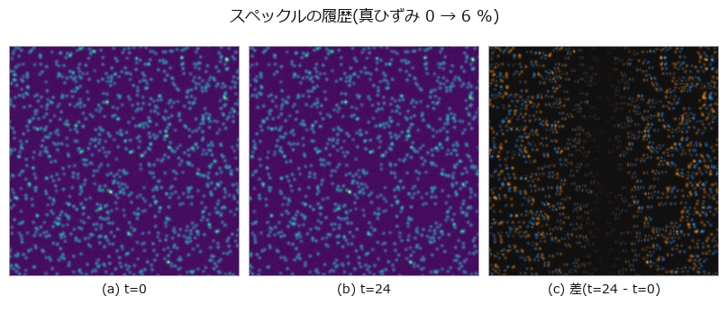
↑ Strain History in a Creep Test — Cumulative or Direct? ―― One hour of creep in 25 frames, with strain history from accumulating adjacent-frame displacements versus comparing each frame directly with the reference. At the end, cumulative errs by 61 µε and direct by 1878 µε — cumulative wins 31x and the textbook crossover in time never appears (it lives on the noise axis instead). Thinning from 24 to 4 steps worsens cumulative from -60 to -606 µε; what matters is the deformation per step, not the number of steps.
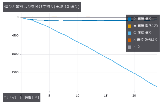
↑ The measurement ―― 直接の偏りだけが伸びる。累積は偏りも散らばりも頭打ちで、しかも散らばりより偏りのほうが大きい ——ランダムウォークではない。 (figure labels are in Japanese; the numbers are the same)
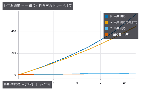
↑ 因果フィルタの偏りは遅れ (w-1)/2 の閉形式にほぼ乗る。
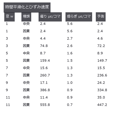
↑ 予測 = w=1 の偏り + 閉形式(中央はなまり、因果は遅れ)。
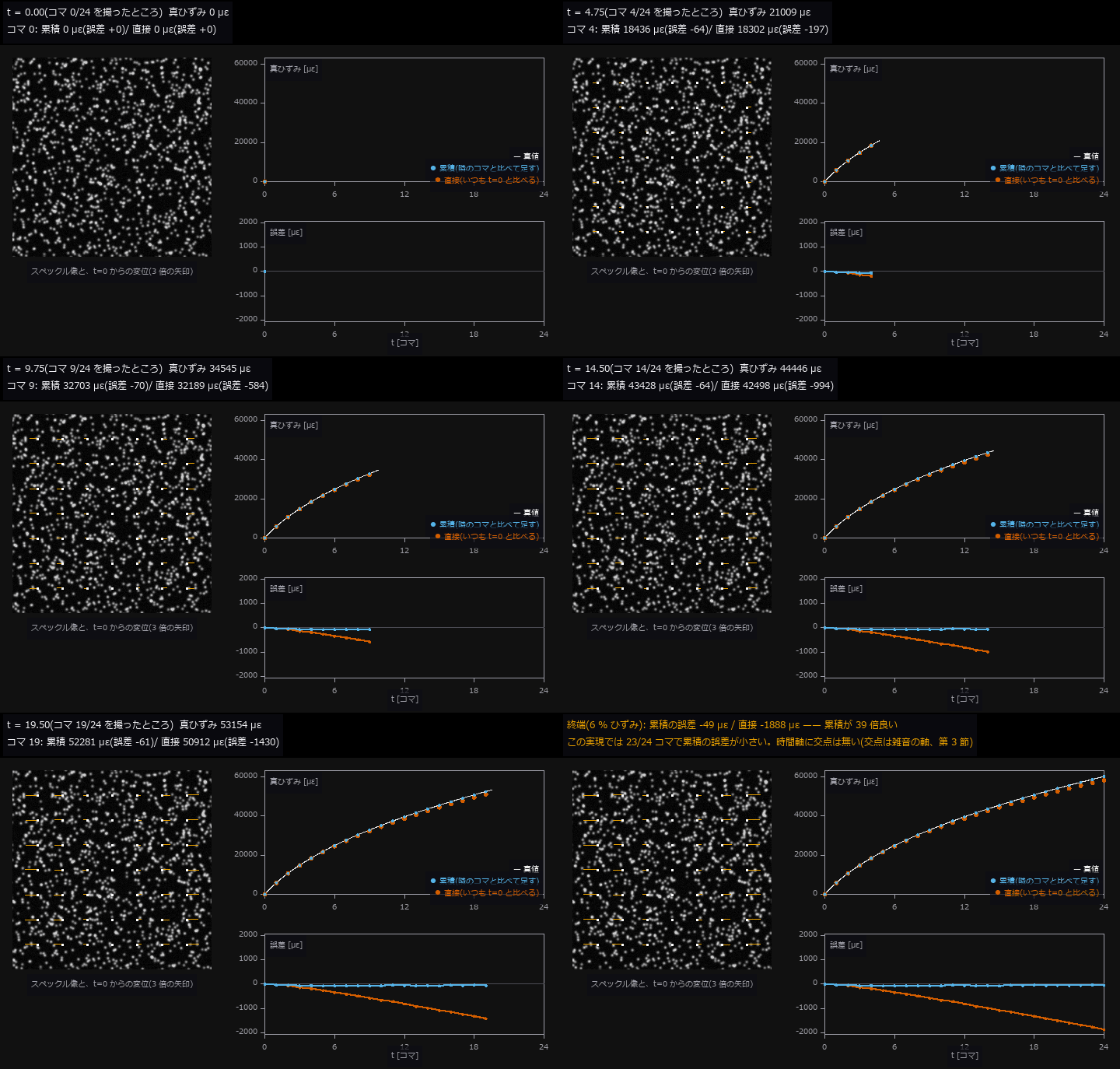
↑ The animation ―― 動画(720 × 458、8 fps、127 コマ): クリープ試験を 25 コマ撮る。左はその時刻のスペックル像に、t=0 との直接 PIV の変位を 3 倍の矢印で重ねたもの(中心から外へ伸びる)。右上は真ひずみ(白、閉形式)と測った値(青 = 隣のコマどうしの増分を足す累積、朱 = いつも t=0 と比べる直接)、右下はその誤差。直接の誤差だけが変形とともに伸び、終端で 累積 -49 µε / 直接 -1888 µε(雑音の実現 1 通り、第 2 節と同じ種)。
py -3.11 examples/poc_strain_history.py
Source: examples/poc_strain_history.py
This run produced 5 figures in total - see them all
Ops used (notes): axes_frame · axes_transform · data_to_pixel · moving_average_window · piv_cross_correlate · piv_error_stats · piv_multipass · piv_sample_at_windows · piv_synth_pair · poly_fit · text_box · ticks
No.2026.040 —— How Far Sa / Sq / Sz Survive Sampling and Cutoff
A prescribed-PSD synthetic surface is measured. Raw rms overstates Sq 20 times; plane removal still leaves 1.8 times. At 8 micrometre sampling Sa is -3.5% and Sz -19.8%. Sq changes little only for this setup; decimation does not generally preserve the second moment. Sz did not plateau over tested areas. Full-length peak-to-valley is Rt, not standardised Rz.
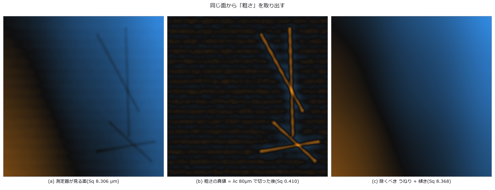
↑ How Far Sa / Sq / Sz Survive Sampling and Cutoff ―― A prescribed-PSD synthetic surface is measured. Raw rms overstates Sq 20 times; plane removal still leaves 1.8 times. At 8 micrometre sampling Sa is -3.5% and Sz -19.8%. Sq changes little only for this setup; decimation does not generally preserve the second moment. Sz did not plateau over tested areas. Full-length peak-to-valley is Rt, not standardised Rz.
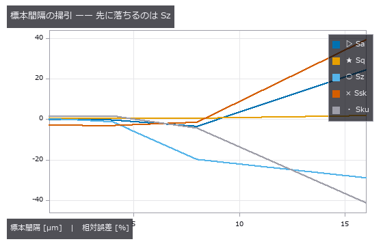
↑ The measurement ―― dx=8 µm では Sa が ±5 % 合格で Sz が不合格。同じデータでも見るパラメータで結論が反転する。 (figure labels are in Japanese; the numbers are the same)
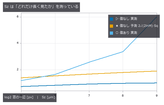
↑ 頭打ちにならないので『真の Sz』は存在しない。
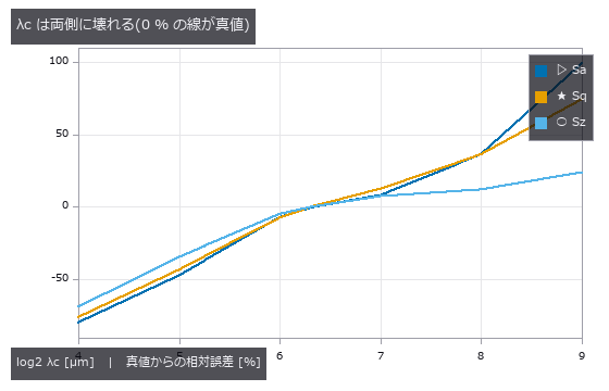
↑ 左は加工目(λ=32µm)を落として過小、右はうねり(λ=256µm)が漏れて過大。
py -3.11 examples/poc_surface_roughness.py
Source: examples/poc_surface_roughness.py
This run produced 4 figures in total - see them all
Ops used (notes): profile_params · surface_filter · surface_form_remove · surface_params · surface_psd · surface_synth_psd
No.2026.196 —— A Vision-Based Tactile Sensor (Elastic Membrane + Camera), Synthesised and Inverted — Hertz Contact and Photometric Stereo in Closed Form as the Gate, Force Read from a Pressed Sphere
| The second exhibit of the physics-simulation × Fullseye series (‘home-made traps have a ceiling: bring in the truth, the gate or the subject from outside’). Two closed-form systems come from outside. Elastic contact: Hertz (Johnson, Contact Mechanics, CUP 1985: a³ = 3FR/(4E), δ = a²/R, p(r) = p0√(1 − r²/a²), half-space surface displacement δ − r²/(2R) inside and eq. 3.42a outside, value δ/2 and slope −a/R both continuous at r = a). Optics: Woodham’s 1980 photometric stereo N = L⁻¹I and the Frankot–Chellappa 1988 normal integration (the principle of reading normals from one image of an elastic membrane lit by three coloured directional lights is Johnson & Adelson, CVPR 2009). Three things are our own: the closed-form radial slope of the outer solution, dh/dr = (2/πR)[r arcsin(a/r) − a√(1 − a²/r²)] (derived; matches numerical differentiation to 5e-9), an inversion that fits this one-parameter Hertz slope model to the radial slope profile of the recovered normal field (it never integrates heights, so FFT amplitude damping, the finite window and the unknown offset do not enter), and a window-truncation correction that adds the Boussinesq far-field tail ū_z ≈ F/(πEr) as r_max·s̄(r_max) to the 1-D slope integral for δ. The subjects are Fullseye’s existing ops (photometric_stereo / integrate_normals / surface_normals / render_lambertian, measure.fit_circle). New module tacsim, 14 ops. Figures: a 1:1 crop around the indentation (62.5 µm/px, a = 0.88 mm = 14 px), synthetic images and recovered heights for a sphere, a cylinder, a straight edge and an ‘F’ stamp, a GIF ramping the load 0.005 → 0.12 N (left the synthetic image, right the Hertz a–F curve filling with points), the recovered-vs-truth cross-section, the slope profile against the Hertz model, a–F with both readouts, and where it breaks (mis-calibration, noise). 17 gates: limits of the combined modulus, Hertz identities (1e-9), pressure integrals equal F and F/L (0.1 %), inner/outer continuity of the surface displacement and the slope derivation, Frankot–Chellappa round trip 0.11 µm (δ = 261 µm), Woodham exactness (median 0.0001°), the fit route a 0.05–0.26 % and F 0.14–0.79 % (0.02–0.12 N), the δ route δ 0.28–0.84 % and F 0.43–1.26 %, the model-free ring −8.2 to −4.9 % (within 1 pt of the resolution prediction −0.7 px/a = −7.8 to −4.3 %), a ∝ F^{1/3} (exponent 0.3335), window truncation deficit 4.37 % (closed form ū_z(r_max)/δ = 4.7 %), not subtracting the ambient 0.03 reads δ 3.17 % low (predicted ambient/sin 55° = 3.7 %), a 15° elevation mis-calibration spoils only the slopes (0.00° → 5.69°, flat gel 0.05°), pixel noise σ = 0.03 gives 2.7° on normals yet F within 0.5 %, the four shapes round-trip to 0.4–0.6 µm RMS (the stamp 10.8 µm from attached shadows on its 60° walls), the cylinder’s geometric half-width √(2Rd − d²) = 1.308 mm (measured 1.312), and tac_contact_mask has recall 0.92 but 1.78× the area. Honestly: small-strain Hertz (δ/R ≈ 0.09), Lambertian, no shadows or speculars, a semi-infinite membrane, no viscoelasticity or markers. The model-free ring sits 5 % inside at a = 14 px (the fit route is primary, the ring is the second implementation). Traps: a thresholded | ∇h | band sits 9 % inside because the cusp is asymmetric, FFT integration damps a deep local dimple by 13 %, and the ambient term tilts normals 3.7 % toward flat (the subtraction that a real sensor’s reference frame provides is needed). Gates alone 0.7 s, with figures 12 s. |

| ↑ A Vision-Based Tactile Sensor (Elastic Membrane + Camera), Synthesised and Inverted — Hertz Contact and Photometric Stereo in Closed Form as the Gate, Force Read from a Pressed Sphere ―― The second exhibit of the physics-simulation × Fullseye series (‘home-made traps have a ceiling: bring in the truth, the gate or the subject from outside’). Two closed-form systems come from outside. Elastic contact: Hertz (Johnson, Contact Mechanics, CUP 1985: a³ = 3FR/(4E), δ = a²/R, p(r) = p0√(1 − r²/a²), half-space surface displacement δ − r²/(2R) inside and eq. 3.42a outside, value δ/2 and slope −a/R both continuous at r = a). Optics: Woodham’s 1980 photometric stereo N = L⁻¹I and the Frankot–Chellappa 1988 normal integration (the principle of reading normals from one image of an elastic membrane lit by three coloured directional lights is Johnson & Adelson, CVPR 2009). Three things are our own: the closed-form radial slope of the outer solution, dh/dr = (2/πR)[r arcsin(a/r) − a√(1 − a²/r²)] (derived; matches numerical differentiation to 5e-9), an inversion that fits this one-parameter Hertz slope model to the radial slope profile of the recovered normal field (it never integrates heights, so FFT amplitude damping, the finite window and the unknown offset do not enter), and a window-truncation correction that adds the Boussinesq far-field tail ū_z ≈ F/(πE*r) as r_max·s̄(r_max) to the 1-D slope integral for δ. The subjects are Fullseye’s existing ops (photometric_stereo / integrate_normals / surface_normals / render_lambertian, measure.fit_circle). New module tacsim, 14 ops. Figures: a 1:1 crop around the indentation (62.5 µm/px, a = 0.88 mm = 14 px), synthetic images and recovered heights for a sphere, a cylinder, a straight edge and an ‘F’ stamp, a GIF ramping the load 0.005 → 0.12 N (left the synthetic image, right the Hertz a–F curve filling with points), the recovered-vs-truth cross-section, the slope profile against the Hertz model, a–F with both readouts, and where it breaks (mis-calibration, noise). 17 gates: limits of the combined modulus, Hertz identities (1e-9), pressure integrals equal F and F/L (0.1 %), inner/outer continuity of the surface displacement and the slope derivation, Frankot–Chellappa round trip 0.11 µm (δ = 261 µm), Woodham exactness (median 0.0001°), the fit route a 0.05–0.26 % and F 0.14–0.79 % (0.02–0.12 N), the δ route δ 0.28–0.84 % and F 0.43–1.26 %, the model-free ring −8.2 to −4.9 % (within 1 pt of the resolution prediction −0.7 px/a = −7.8 to −4.3 %), a ∝ F^{1/3} (exponent 0.3335), window truncation deficit 4.37 % (closed form ū_z(r_max)/δ = 4.7 %), not subtracting the ambient 0.03 reads δ 3.17 % low (predicted ambient/sin 55° = 3.7 %), a 15° elevation mis-calibration spoils only the slopes (0.00° → 5.69°, flat gel 0.05°), pixel noise σ = 0.03 gives 2.7° on normals yet F within 0.5 %, the four shapes round-trip to 0.4–0.6 µm RMS (the stamp 10.8 µm from attached shadows on its 60° walls), the cylinder’s geometric half-width √(2Rd − d²) = 1.308 mm (measured 1.312), and tac_contact_mask has recall 0.92 but 1.78× the area. Honestly: small-strain Hertz (δ/R ≈ 0.09), Lambertian, no shadows or speculars, a semi-infinite membrane, no viscoelasticity or markers. The model-free ring sits 5 % inside at a = 14 px (the fit route is primary, the ring is the second implementation). Traps: a thresholded | ∇h | band sits 9 % inside because the cusp is asymmetric, FFT integration damps a deep local dimple by 13 %, and the ambient term tilts normals 3.7 % toward flat (the subtraction that a real sensor’s reference frame provides is needed). Gates alone 0.7 s, with figures 12 s.* |

↑ The measurement ―― 球・円柱・直線エッジ・F 字スタンプを 0.3 mm 押し込んだ膜(幾何学的な追従、弾性の裾なし、46.9 µm/px、中央 ±1.9 mm を 3 倍)。上 = 3 色照明の合成像、下 = フォトメトリックステレオ + Frankot-Chellappa で復元した高さ(接触域の RMS を併記)。 (figure labels are in Japanese; the numbers are the same)

↑ 中央行の断面。
[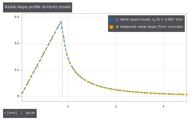](https://raw.githubusercontent.com/furuse-kazufumi/fullseye/master/docs/articles/assets/poc/poc_tacsim_elastic_membrane/05_tacsim_slope_profile_fit.png)
↑ 法線場から取った半径方向スロープの方位平均(点)と、1 パラメータ a で当てた Hertz のスロープ模型(破線: 内側 r/R、外側 (2/πR)[r arcsin(a/r) − a√(1−a²/r²)])。

↑ 破線 = Hertz の閉形式。
[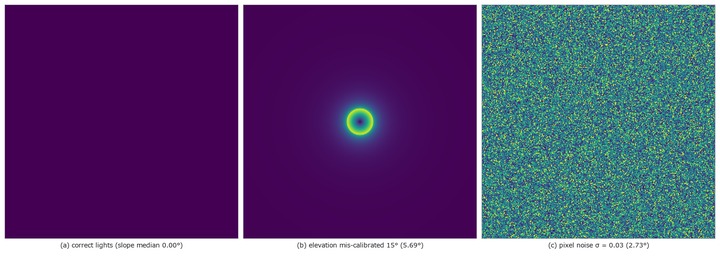](https://raw.githubusercontent.com/furuse-kazufumi/fullseye/master/docs/articles/assets/poc/poc_tacsim_elastic_membrane/07_tacsim_failure_modes.png)
↑ 壊れる場所: 法線の角誤差 [deg]。
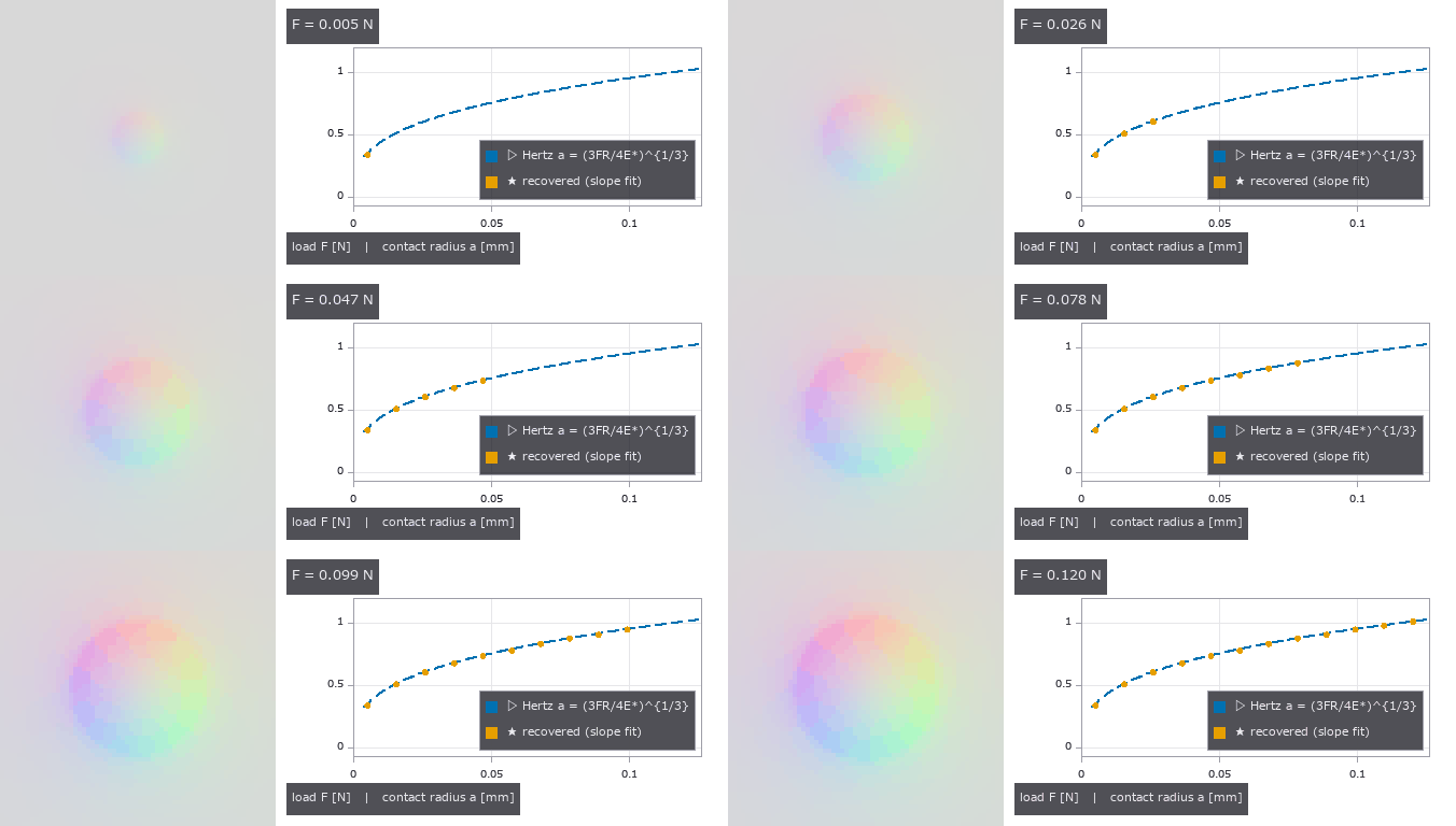
↑ The animation ―― 荷重を 0.005 → 0.12 N に上げる(12 コマ)。左 = 圧痕まわり ±2.0 mm の合成像(62.5 µm/px を 4 倍)、右 = Hertz の a–F 曲線(破線 = 閉形式)に、各コマの像から当てはめ経路で読んだ a が点として増えていく。
py -3.11 examples/poc_tacsim_elastic_membrane.py
Source: examples/poc_tacsim_elastic_membrane.py
This run produced 7 figures in total - see them all
Ops used (notes): combined_modulus · contact_radius_fit · contact_radius_ring · hertz_cylinder · hertz_force · hertz_pressure · hertz_sphere · hertz_surface_uz · integrate_normals · membrane_delta_from_normals · membrane_indent_shape · membrane_indent_sphere · membrane_lights · membrane_recover · membrane_render_rgb · photometric_stereo · tac_contact_mask
No.2026.198 —— Reading the Shear Field, Stick/Slip and Tangential Force from a Tactile Sensor’s Marker Array — Cattaneo–Mindlin in Closed Form and Finite-Element Nodal Displacements as the Gate
| The second exhibit of the second physics-simulation × Fullseye round (the first read force from a normal indentation). Two things come from outside. Closed forms (Johnson, Contact Mechanics, CUP 1985): the Cattaneo 1938 / Mindlin 1949 partial-slip solution (§7.2) — a sphere pressed with normal P and then loaded tangentially with Q < μP has a stick circle c/a = (1 − Q/μP)^{1/3}, a shear traction q = q′ − q″ (the difference of two Hertz-shaped tractions, pinned at the Coulomb limit μp(r) in the slip annulus), a rigid-sphere tangential displacement δx = 3μP(2−ν)/(16Ga)[1 − (1−Q/μP)^{2/3}], an initial tangential stiffness kt = 8Ga/(2−ν), and a uniform surface displacement inside the stick circle; the inner solution for one Hertz-shaped tangential traction (eq. 3.91); the radial surface displacement under normal load (eq. 3.41b); and the Cerruti half-space solution for a tangential point load (eq. 3.22). Finite-element nodal displacements of a finite-thickness dome-shaped gel (shipped with the Robo-Touch/Taxim repository, MIT; used only when FULLSEYE_TAXIM_DATA is set, never copied into the repo). Published qualitative facts (Yuan, Dong & Adelson, Sensors 2017): slip starts at the periphery and the entropy of the marker-displacement histogram rises under partial slip. Three things are our own: outside the contact circle and in the slip annulus there is no closed form, so the Cerruti kernel is discretised as pixel averages (analytic centre pixel, 4h ln(1+√2)) and convolved by FFT (ūx 0.017 % and ūy 0.03 % against eq. 3.91 inside the circle, stick-core uniformity std 0.006 %); a similarity-law inverse model g(x) − (c/a)²g(x·a/c) that yields the field for any stick radius from one convolution (c/a to 0.001 on the true displacements); and marker images drawn by moving the centres before rendering (no interpolation). The subjects are Fullseye’s existing ops: blob2d.blob_label / blob_features (centroids), pivops.piv_cross_correlate (window correlation, second implementation), the sub-pixel extrema of backends_subpix, backends_tactile.tac_shear_field (a separate subject), measure.fit_circle, and tacsim’s Hertz table and membrane rendering. New module tacslip, 20 ops. The dimensions were chosen to kill the resolution trap first: R = 6 mm, P = 0.5 N, E 0.2 MPa, ν 0.48 → a = 2.05 mm = 32.9 px (62.5 µm/px), markers at 0.5 mm = 8 px (radius 2.5 px) giving 53 inside the contact circle, full-slip δx = 514 µm = 8.2 px; μ = 0.5 is an assumption (the value that reproduces the plan’s anchor of 70.5 µm). Figures: a triptych of reference / loaded / tracked vectors (uniform motion inside the stick circle, lag in the slip annulus, a 1/r tail outside), a GIF ramping the tangential force 0 → μP (the closed-form stick circle in green and the fitted c in red coincide, and the core vanishes at full slip), the two terms of q(r), δx–Q (closed-form line and stick-core medians), entropy vs Q/μP, finite elements vs half-space (decay of r·u and the angular form of dx(θ)), and where it breaks (lattice aliasing, density, noise). 20 gates (the two finite-element gates when the data is present; gates alone 2.8 s, with figures 19 s): ∫q dA = Q (6e-7), the closed-form c/a and the full-slip flag, dδx/dQ(0) = 1/kt (1e-6) and the 70.6 µm anchor, ūr(a)/δ = 2(1−2ν)/(3π(1−ν)) = 1.6 % (derived), the Cerruti convolution against eq. 3.91, stick-core uniformity, the far field 1/r (1.016 at 3a), the centroid round trip (iterated Gaussian-weighted 0.003 px, binary 0.16 px, lattice-wide common bias 0.010 → 0.004 px), markers move at most 0.187 px under the normal load alone = the maximum of | ūr | (at r = 0.93a, 1.022 × ūr(a)), tracking RMS 0.007–0.010 px (Q/μP 0.25–0.9, 961/961 matched), PIV reads a 5 px shift of an 8 px lattice as −3.000 px (4.999 on a jittered lattice) and agrees to 0.03 px in the stick core once the search is capped at ±3.8 px, the inversion’s Q/μP error 0.026 → 0.007, c/a 0.011, Q 0.4–0.9 %, μ 10.2 → 1.2 % (μ and Q separate once G, ν and a are known, but the error in μ is the error in c/a amplified by 2c/(1−c²) = 10.4 → 1.2), the model-free stick radius 2.3–4.7 px (= the marker pitch), c/a 0.000 and a 42 % spread of the core at full slip, exponent 0.341 (closed form 1/3), entropy 0.078 → 0.677 non-decreasing, tac_shear_field does not separate stick from slip (core 0.043, annulus 0.039), Q/μP within 0.03 even at a 16 px pitch (13 markers inside) and tracking RMS 0.031 px at pixel noise σ 0.05, and for the finite elements r·dz falls to half of the 1/r law at r½ = 2.27 mm (0.88 at 1 mm, 0.57 at 2 mm, 0.32 at 3 mm) while dx(θ) at r = 1.5–2 mm follows Cerruti’s A + B cos²θ (R² 0.78–0.80) with ν 0.49–0.51 and exceeds the half-space bound of 2 at r = 3 mm (2.4). Honestly: half-space, small strain, rigid sphere, Coulomb friction, quasi-static (no time evolution of incipient slip, no viscoelasticity; the shear strain near the edge approaches 0.25 at full slip, outside linear elasticity), μ is poorly determined at low Q (10 % at Q/μP 0.25), the finite-element data is a point-like load (contact smaller than the 0.16 mm node spacing) with unknown force so the stick circle cannot be tested and only shapes are compared (even the normal-load case carries dy/dz = 0.25 of asymmetry), correlation and nearest-neighbour matching cannot in principle measure | u | ≥ pitch/2 (the matching relies on the image border being far field), and 53 markers quantise the entropy. Traps: correlation on a regular lattice aliases at the lattice period (a 64→32 multipass jumps to ±8/±16 in its first pass), the 6.4 px core displacement lands 1.6 px from the neighbouring reference position so even nearest-neighbour seeds jump (hence growing the matching inward from the border), the centroid of a 2 px disc carries ±0.03 px of pixel-locking that becomes a lattice-wide common mode and shifts c/a by 0.02 (a 2.5 px radius plus iterated Gaussian weights cut it to a third; a free rigid-shift term is degenerate with the 1/r tail and makes it worse), the maximum of ūr sits inside the edge at 0.93a, neighbouring marker fringes merge in the slip annulus as the spacing shrinks from 8 to 6 px, and a model that interpolates fields on a c/a grid is off by 0.01. δx_full ≈ marker pitch is the worst pairing — a real sensor wants pitch > 2·δx_full or an aperiodic layout. |

| *↑ Reading the Shear Field, Stick/Slip and Tangential Force from a Tactile Sensor’s Marker Array — Cattaneo–Mindlin in Closed Form and Finite-Element Nodal Displacements as the Gate ―― The second exhibit of the second physics-simulation × Fullseye round (the first read force from a normal indentation). Two things come from outside. Closed forms (Johnson, Contact Mechanics, CUP 1985): the Cattaneo 1938 / Mindlin 1949 partial-slip solution (§7.2) — a sphere pressed with normal P and then loaded tangentially with Q < μP has a stick circle c/a = (1 − Q/μP)^{1/3}, a shear traction q = q′ − q″ (the difference of two Hertz-shaped tractions, pinned at the Coulomb limit μp(r) in the slip annulus), a rigid-sphere tangential displacement δx = 3μP(2−ν)/(16Ga)[1 − (1−Q/μP)^{2/3}], an initial tangential stiffness kt = 8Ga/(2−ν), and a uniform surface displacement inside the stick circle; the inner solution for one Hertz-shaped tangential traction (eq. 3.91); the radial surface displacement under normal load (eq. 3.41b); and the Cerruti half-space solution for a tangential point load (eq. 3.22). Finite-element nodal displacements of a finite-thickness dome-shaped gel (shipped with the Robo-Touch/Taxim repository, MIT; used only when FULLSEYE_TAXIM_DATA is set, never copied into the repo). Published qualitative facts (Yuan, Dong & Adelson, Sensors 2017): slip starts at the periphery and the entropy of the marker-displacement histogram rises under partial slip. Three things are our own: outside the contact circle and in the slip annulus there is no closed form, so the Cerruti kernel is discretised as pixel averages (analytic centre pixel, 4h ln(1+√2)) and convolved by FFT (ūx 0.017 % and ūy 0.03 % against eq. 3.91 inside the circle, stick-core uniformity std 0.006 %); a similarity-law inverse model g(x) − (c/a)²g(x·a/c) that yields the field for any stick radius from one convolution (c/a to 0.001 on the true displacements); and marker images drawn by moving the centres before rendering (no interpolation). The subjects are Fullseye’s existing ops: blob2d.blob_label / blob_features (centroids), pivops.piv_cross_correlate (window correlation, second implementation), the sub-pixel extrema of backends_subpix, backends_tactile.tac_shear_field (a separate subject), measure.fit_circle, and tacsim’s Hertz table and membrane rendering. New module tacslip, 20 ops. The dimensions were chosen to kill the resolution trap first: R = 6 mm, P = 0.5 N, E 0.2 MPa, ν 0.48 → a = 2.05 mm = 32.9 px (62.5 µm/px), markers at 0.5 mm = 8 px (radius 2.5 px) giving 53 inside the contact circle, full-slip δx = 514 µm = 8.2 px; μ = 0.5 is an assumption (the value that reproduces the plan’s anchor of 70.5 µm). Figures: a triptych of reference / loaded / tracked vectors (uniform motion inside the stick circle, lag in the slip annulus, a 1/r tail outside), a GIF ramping the tangential force 0 → μP (the closed-form stick circle in green and the fitted c in red coincide, and the core vanishes at full slip), the two terms of q(r), δx–Q (closed-form line and stick-core medians), entropy vs Q/μP, finite elements vs half-space (decay of r·u and the angular form of dx(θ)), and where it breaks (lattice aliasing, density, noise). 20 gates (the two finite-element gates when the data is present; gates alone 2.8 s, with figures 19 s): ∫q dA = Q (6e-7), the closed-form c/a and the full-slip flag, dδx/dQ(0) = 1/kt (1e-6) and the 70.6 µm anchor, ūr(a)/δ = 2(1−2ν)/(3π(1−ν)) = 1.6 % (derived), the Cerruti convolution against eq. 3.91, stick-core uniformity, the far field 1/r (1.016 at 3a), the centroid round trip (iterated Gaussian-weighted 0.003 px, binary 0.16 px, lattice-wide common bias 0.010 → 0.004 px), markers move at most 0.187 px under the normal load alone = the maximum of | ūr | (at r = 0.93a, 1.022 × ūr(a)), tracking RMS 0.007–0.010 px (Q/μP 0.25–0.9, 961/961 matched), PIV reads a 5 px shift of an 8 px lattice as −3.000 px (4.999 on a jittered lattice) and agrees to 0.03 px in the stick core once the search is capped at ±3.8 px, the inversion’s Q/μP error 0.026 → 0.007, c/a 0.011, Q 0.4–0.9 %, μ 10.2 → 1.2 % (μ and Q separate once G, ν and a are known, but the error in μ is the error in c/a amplified by 2c/(1−c²) = 10.4 → 1.2), the model-free stick radius 2.3–4.7 px (= the marker pitch), c/a 0.000 and a 42 % spread of the core at full slip, exponent 0.341 (closed form 1/3), entropy 0.078 → 0.677 non-decreasing, tac_shear_field does not separate stick from slip (core 0.043, annulus 0.039), Q/μP within 0.03 even at a 16 px pitch (13 markers inside) and tracking RMS 0.031 px at pixel noise σ 0.05, and for the finite elements r·dz falls to half of the 1/r law at r½ = 2.27 mm (0.88 at 1 mm, 0.57 at 2 mm, 0.32 at 3 mm) while dx(θ) at r = 1.5–2 mm follows Cerruti’s A + B cos²θ (R² 0.78–0.80) with ν 0.49–0.51 and exceeds the half-space bound of 2 at r = 3 mm (2.4). Honestly: half-space, small strain, rigid sphere, Coulomb friction, quasi-static (no time evolution of incipient slip, no viscoelasticity; the shear strain near the edge approaches 0.25 at full slip, outside linear elasticity), μ is poorly determined at low Q (10 % at Q/μP 0.25), the finite-element data is a point-like load (contact smaller than the 0.16 mm node spacing) with unknown force so the stick circle cannot be tested and only shapes are compared (even the normal-load case carries dy/dz = 0.25 of asymmetry), correlation and nearest-neighbour matching cannot in principle measure | u | ≥ pitch/2 (the matching relies on the image border being far field), and 53 markers quantise the entropy. Traps: correlation on a regular lattice aliases at the lattice period (a 64→32 multipass jumps to ±8/±16 in its first pass), the 6.4 px core displacement lands 1.6 px from the neighbouring reference position so even nearest-neighbour seeds jump (hence growing the matching inward from the border), the centroid of a 2 px disc carries ±0.03 px of pixel-locking that becomes a lattice-wide common mode and shifts c/a by 0.02 (a 2.5 px radius plus iterated Gaussian weights cut it to a third; a free rigid-shift term is degenerate with the 1/r tail and makes it worse), the maximum of ūr sits inside the edge at 0.93a, neighbouring marker fringes merge in the slip annulus as the spacing shrinks from 8 to 6 px, and a model that interpolates fields on a c/a grid is off by 0.01. δx_full ≈ marker pitch is the worst pairing — a real sensor wants pitch > 2·δx_full or an aperiodic layout.* |
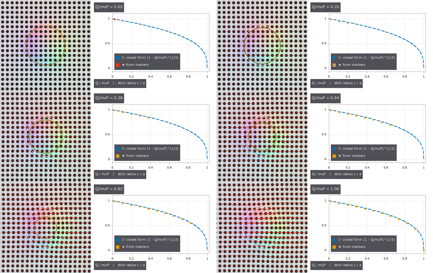
↑ The measurement ―― 接線力を 0 → μP に上げる(12 コマ)。左 = マーカー像 + 追跡ベクトル(4 倍)、緑 = 閉形式の固着円 c = a(1 − Q/μP)^{1/3}、赤 = 画像から当てた c、白 = 接触円 a。右 = c/a の閉形式(破線)に各コマの推定点が増える。Q = μP で核が消え全滑り。 (figure labels are in Japanese; the numbers are the same)
[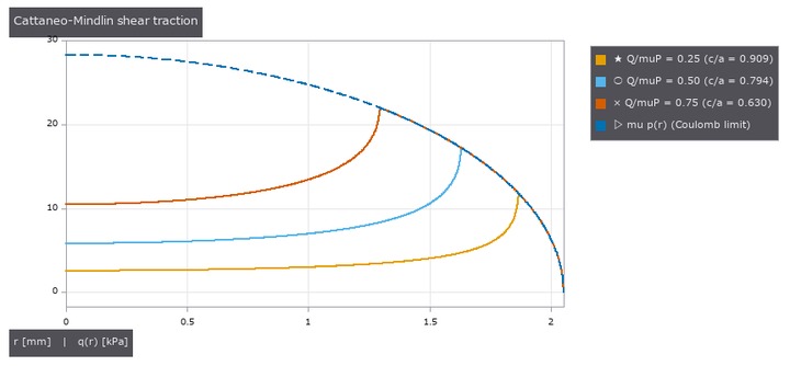](https://raw.githubusercontent.com/furuse-kazufumi/fullseye/master/docs/articles/assets/poc/poc_tacsim_marker_shear/03_tacslip_traction_q_r.png)
↑ 接線トラクション q(r) = μp0[√(1−r²/a²) − (c/a)√(1−r²/c²)]。
[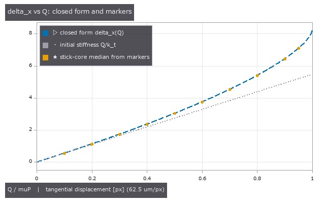](https://raw.githubusercontent.com/furuse-kazufumi/fullseye/master/docs/articles/assets/poc/poc_tacsim_marker_shear/04_tacslip_delta_x_vs_Q.png)
↑ 剛体球の接線変位 δx = 3μP(2−ν)/(16Ga)[1 − (1−Q/μP)^{2/3}] (破線)と初期剛性 kt = 8Ga/(2−ν) の直線(点線)。

↑ 接触円内のマーカー変位の大きさのヒストグラム(16 ビン)のエントロピー。

↑ 第 2 真値: 有限要素の節点変位(ドーム状の有限厚ゲル、Robo-Touch/Taxim リポジトリ同梱、MIT)と半空間解。
py -3.11 examples/poc_tacsim_marker_shear.py
Source: examples/poc_tacsim_marker_shear.py
This run produced 7 figures in total - see them all
Ops used (notes): blob_features · cerruti_kernel · cerruti_surface_displacement · combined_modulus · displace_markers · fem_nodes_load · fem_vs_halfspace · hertz_pressure · hertz_sphere · hertz_surface_ur · hertzian_tangential_inner · marker_detect · marker_image · marker_track · membrane_indent_sphere · membrane_lights · membrane_markers · membrane_render_markers · membrane_render_rgb · membrane_shear_field · mindlin_fit · mindlin_model · mindlin_partial_slip · mindlin_traction … (+5)
No.2026.199 —— Reading In-Grasp Tilt and Torsion Torque from a Tactile Sensor’s Marker Field with a ‘Tactile Dipole’ — Gauss’s Law Becoming an Identity in the Half-Space as the Gate
| The third exhibit of the second physics-simulation × Fullseye round (the first read force from a normal indentation, the second shear and stick/slip from a marker array). The re-implemented method is Fuchioka & Hamaya, ICRA 2024 (arXiv 2404.15626): learning-free and optics-free, it treats the divergence ∇·v of the marker displacement field as a ‘charge’ (the normal-force distribution, by analogy with Gauss’s law), takes the dipole p = (1/N) Σ r_i (∇·v)_i about the midpoint of the positive and negative charge centroids, and reads the tilt torque orthogonal to the dipole, τ = [c_x p_y, −c_y p_x], with c calibrated linearly against a force sensor. The essential step is zeroing after the grasp. The authors’ code has no licence, so it was never read; everything comes from the equations in the paper. The sensor family is retrographic sensing (Johnson & Adelson 2009). Two things come from outside. Closed forms (Johnson, Contact Mechanics, CUP 1985): the pressure under a flat circular punch p = P/(2πa√(a²−r²)) (eq. 3.34) plus the antisymmetric term 3Mx/(2πa³√(a²−r²)) for a tilting moment (∫ x p dA = M, no lift-off for M ≤ Pa/3, derived), the Boussinesq half-space surface displacements of a normal point load (§3.2: ū_r = −(1−2ν)P/(4πGr), ū_z = (1−ν)P/(2πGr)), the surface displacements of a Hertz pressure (eqs. 3.41b, 3.42a), the elliptical Hertz pressure (eq. 4.24), no-slip torsion (Reissner–Sagoci) q_θ = 3M_z r/(4πa³√(a²−r²)) with β = 3M_z/(16Ga³), and the Cattaneo–Mindlin partial slip of the previous exhibit. Finite-element nodal displacements of a finite-thickness dome-shaped gel (shipped with the Robo-Touch/Taxim repository, MIT; used only when FULLSEYE_TAXIM_DATA is set, never copied into the repo). Three things are our own derivations, all turned into gates: Gauss’s law is exact in the half-space — since ∇·(r̂/r) = 2πδ² in two dimensions, ∇·ū = −(1−2ν)p/(2G), so the area-weighted dipole is proportional to the first moment of pressure (= the tilt moment M) regardless of the indenter’s shape (but the coefficient −(1−2ν)/(2G) vanishes as ν → 0.5: a real sensor’s signal comes from the bulging of the finite-thickness gel); the divergence of the Cerruti point-load field, −(1−ν)Qx/(2πGr³) — a pure shear produces a false tilt of (1−ν)/(1−2ν)·Q·R over the whole window (13·Q·R at ν 0.48), so the window is limited to the stick circle (the tilt charge concentrates at the edge singularity and wants a window ≥ a + 1.5 pitch; the two cannot both hold, so a small window gives a fixed fraction 0.47 that calibration absorbs); and the baseline form ( | u | as charge) is identically zero for a zeroed symmetric tilt because | u | is even in M. The subjects are existing ops: tacslip.marker_track (centroids and matching), the tacslip.cerruti_kernel convolution (an independent implementation of torsion), sceneflow.flow_divergence / flow_curl (second implementation on the grid), pivops.piv_vorticity (−curl under its (dy, dx) convention). New module tactorque, 17 ops. Dimensions: flat punch a = 3 mm, P = 2 N (lift-off at M = 2 N·mm), 16 mm field, 128 px gate grid (125 µm/px), 256 px image grid (62.5 µm/px), 0.5 mm markers. Figures: marker image + tracked vectors (×40) + dipole arrow (1:1 crop) with the divergence map of the tracked field, a GIF ramping M 0 → 1.5 N·mm (the dipole grows and the points land on the closed-form line), the decomposition maps (divergence → tilt, curl → torsion, mean → translation), FEM normal vs oblique (divergence scatter + radial profile), where it breaks (noise ∝ σ, a shear leak that moves six decades with the window radius, −57 % for a window 2 mm off-centre), and the coefficient for three shapes. 17 gates (the two FEM gates when the data is present; measured without the FEM data, gates alone 2.0 s, with figures 29 s): grid integrals of the punch pressure Σp h² = P to 0.57 % and Σx p h² = M to 0.86 % (the 1/√ edge) and the lift-off fail-closed, the Boussinesq kernel against 3.41b (0.03 %), 3.42a (0.01 %) and the punch u_z (0.35 %), the Gauss identity to 0.21 % (identical at ν 0.48 and 0.3, confirming the (1−2ν) scaling), zero dipole under pure normal load (8e-16, three forms), D ∝ M with R² = 1.000000, the coefficient within 0.035 % of the closed form, D_y/D_x 4e-4 and origin independence 1e-4 (net lattice charge −8e-4), the baseline form 3e-4, a coefficient spread over punch / sphere / ridge of 0.001 % dense and 0.25 % on the 0.5 mm lattice, torsion ∫r q dA = M_z 0.99, β −0.47 %, uniformity 0.14 %, rigid rotation −0.5 %, curl −0.5 %, piv_vorticity = −curl to 1e-16 (the flat punch’s q/(μp) peaks at 0.238, so no-slip is exact there), a Hertz contact’s partial-slip twist at 0.5 / 0.8 of full slip read by the default to ×0.999 / ×1.000 where the 0.4.0 no-slip relation over-reads ×1.330 / ×1.851 (fixed on 2026-10-06: the old gates synthesised and read with the same no-slip model, so they could not see it), the superposed decomposition (tilt 2.35 % with torsion→tilt cross-talk, 0.22 % alone; torsion 0.5 %; translation 0.038 px), the pure-shear leak ≤ 0.0012 N·mm inside the stick circle minus the fit radius vs 32.5 N·mm over the full window (derived 31.2), centroid noise 0.03 px → σ_M = 0.114 N·mm (window 1.5a, 252 markers), 0.72 over the full window and 0.038 at 0.01 px (∝ σ), 11/11 spelling-breaks plus nan-not-zero, scattered least squares = central differences to 1e-15 (5 points; the 9-point fit differs by 11 % at the edge), the image pipeline (M1 error 0.7 %, tracking RMS 0.0054 px, 961/961 matched), and the FEM: core divergence +0.019 with a ring of −0.0036 (bulging, opposite in sign to the half-space) and an oblique-load dipole ΔD_x = −6.4e-11 m³ for Δt_x = +19 µm (the shear-leak sign). Honestly: the half-space coefficient does not give the magnitude on a real (finite, nearly incompressible) gel — 1 N·mm is 0.06 px at ν 0.48, the same position as the paper’s calibration; three Johnson equation numbers (tilted punch, punch u_z, Reissner–Sagoci) were not checked against the text and are verified numerically by independent implementations; Lubkin’s 1951 closed form for partial-slip torsion is not implemented (partial slip is corrected with cuttouch’s numerical solution); the paper’s per-object calibration factors are a finite-thickness effect (the half-space is shape-free) and no real sensor was tested here; viscoelasticity, the time evolution of incipient slip and optical flow are out of scope. Traps: the 9-point (3×3) plane fit is a row-averaged difference and is 11 % off at the edge (5 points reproduce central differences), the mean curl/2 is 11 % low at the edge (hence the rigid-rotation least squares), torsion picks up the sub-pixel lattice phase and leaks 2 % into tilt, and the origin-independence gate breaks at the lattice’s net charge of 1e-3, so its threshold is 1e-3 rather than 1e-6. |

| *↑ Reading In-Grasp Tilt and Torsion Torque from a Tactile Sensor’s Marker Field with a ‘Tactile Dipole’ — Gauss’s Law Becoming an Identity in the Half-Space as the Gate ―― The third exhibit of the second physics-simulation × Fullseye round (the first read force from a normal indentation, the second shear and stick/slip from a marker array). The re-implemented method is Fuchioka & Hamaya, ICRA 2024 (arXiv 2404.15626): learning-free and optics-free, it treats the divergence ∇·v of the marker displacement field as a ‘charge’ (the normal-force distribution, by analogy with Gauss’s law), takes the dipole p = (1/N) Σ r_i (∇·v)_i about the midpoint of the positive and negative charge centroids, and reads the tilt torque orthogonal to the dipole, τ = [c_x p_y, −c_y p_x], with c calibrated linearly against a force sensor. The essential step is zeroing after the grasp. The authors’ code has no licence, so it was never read; everything comes from the equations in the paper. The sensor family is retrographic sensing (Johnson & Adelson 2009). Two things come from outside. Closed forms (Johnson, Contact Mechanics, CUP 1985): the pressure under a flat circular punch p = P/(2πa√(a²−r²)) (eq. 3.34) plus the antisymmetric term 3Mx/(2πa³√(a²−r²)) for a tilting moment (∫ x p dA = M, no lift-off for M ≤ Pa/3, derived), the Boussinesq half-space surface displacements of a normal point load (§3.2: ū_r = −(1−2ν)P/(4πGr), ū_z = (1−ν)P/(2πGr)), the surface displacements of a Hertz pressure (eqs. 3.41b, 3.42a), the elliptical Hertz pressure (eq. 4.24), no-slip torsion (Reissner–Sagoci) q_θ = 3M_z r/(4πa³√(a²−r²)) with β = 3M_z/(16Ga³), and the Cattaneo–Mindlin partial slip of the previous exhibit. Finite-element nodal displacements of a finite-thickness dome-shaped gel (shipped with the Robo-Touch/Taxim repository, MIT; used only when FULLSEYE_TAXIM_DATA is set, never copied into the repo). Three things are our own derivations, all turned into gates: Gauss’s law is exact in the half-space — since ∇·(r̂/r) = 2πδ² in two dimensions, ∇·ū = −(1−2ν)p/(2G), so the area-weighted dipole is proportional to the first moment of pressure (= the tilt moment M) regardless of the indenter’s shape (but the coefficient −(1−2ν)/(2G) vanishes as ν → 0.5: a real sensor’s signal comes from the bulging of the finite-thickness gel); the divergence of the Cerruti point-load field, −(1−ν)Qx/(2πGr³) — a pure shear produces a false tilt of (1−ν)/(1−2ν)·Q·R over the whole window (13·Q·R at ν 0.48), so the window is limited to the stick circle (the tilt charge concentrates at the edge singularity and wants a window ≥ a + 1.5 pitch; the two cannot both hold, so a small window gives a fixed fraction 0.47 that calibration absorbs); and the baseline form ( | u | as charge) is identically zero for a zeroed symmetric tilt because | u | is even in M. The subjects are existing ops: tacslip.marker_track (centroids and matching), the tacslip.cerruti_kernel convolution (an independent implementation of torsion), sceneflow.flow_divergence / flow_curl (second implementation on the grid), pivops.piv_vorticity (−curl under its (dy, dx) convention). New module tactorque, 17 ops. Dimensions: flat punch a = 3 mm, P = 2 N (lift-off at M = 2 N·mm), 16 mm field, 128 px gate grid (125 µm/px), 256 px image grid (62.5 µm/px), 0.5 mm markers. Figures: marker image + tracked vectors (×40) + dipole arrow (1:1 crop) with the divergence map of the tracked field, a GIF ramping M 0 → 1.5 N·mm (the dipole grows and the points land on the closed-form line), the decomposition maps (divergence → tilt, curl → torsion, mean → translation), FEM normal vs oblique (divergence scatter + radial profile), where it breaks (noise ∝ σ, a shear leak that moves six decades with the window radius, −57 % for a window 2 mm off-centre), and the coefficient for three shapes. 17 gates (the two FEM gates when the data is present; measured without the FEM data, gates alone 2.0 s, with figures 29 s): grid integrals of the punch pressure Σp h² = P to 0.57 % and Σx p h² = M to 0.86 % (the 1/√ edge) and the lift-off fail-closed, the Boussinesq kernel against 3.41b (0.03 %), 3.42a (0.01 %) and the punch u_z (0.35 %), the Gauss identity to 0.21 % (identical at ν 0.48 and 0.3, confirming the (1−2ν) scaling), zero dipole under pure normal load (8e-16, three forms), D ∝ M with R² = 1.000000, the coefficient within 0.035 % of the closed form, D_y/D_x 4e-4 and origin independence 1e-4 (net lattice charge −8e-4), the baseline form 3e-4, a coefficient spread over punch / sphere / ridge of 0.001 % dense and 0.25 % on the 0.5 mm lattice, torsion ∫r q dA = M_z 0.99, β −0.47 %, uniformity 0.14 %, rigid rotation −0.5 %, curl −0.5 %, piv_vorticity = −curl to 1e-16 (the flat punch’s q/(μp) peaks at 0.238, so no-slip is exact there), a Hertz contact’s partial-slip twist at 0.5 / 0.8 of full slip read by the default to ×0.999 / ×1.000 where the 0.4.0 no-slip relation over-reads ×1.330 / ×1.851 (fixed on 2026-10-06: the old gates synthesised and read with the same no-slip model, so they could not see it), the superposed decomposition (tilt 2.35 % with torsion→tilt cross-talk, 0.22 % alone; torsion 0.5 %; translation 0.038 px), the pure-shear leak ≤ 0.0012 N·mm inside the stick circle minus the fit radius vs 32.5 N·mm over the full window (derived 31.2), centroid noise 0.03 px → σ_M = 0.114 N·mm (window 1.5a, 252 markers), 0.72 over the full window and 0.038 at 0.01 px (∝ σ), 11/11 spelling-breaks plus nan-not-zero, scattered least squares = central differences to 1e-15 (5 points; the 9-point fit differs by 11 % at the edge), the image pipeline (M1 error 0.7 %, tracking RMS 0.0054 px, 961/961 matched), and the FEM: core divergence +0.019 with a ring of −0.0036 (bulging, opposite in sign to the half-space) and an oblique-load dipole ΔD_x = −6.4e-11 m³ for Δt_x = +19 µm (the shear-leak sign). Honestly: the half-space coefficient does not give the magnitude on a real (finite, nearly incompressible) gel — 1 N·mm is 0.06 px at ν 0.48, the same position as the paper’s calibration; three Johnson equation numbers (tilted punch, punch u_z, Reissner–Sagoci) were not checked against the text and are verified numerically by independent implementations; Lubkin’s 1951 closed form for partial-slip torsion is not implemented (partial slip is corrected with cuttouch’s numerical solution); the paper’s per-object calibration factors are a finite-thickness effect (the half-space is shape-free) and no real sensor was tested here; viscoelasticity, the time evolution of incipient slip and optical flow are out of scope. Traps: the 9-point (3×3) plane fit is a row-averaged difference and is 11 % off at the edge (5 points reproduce central differences), the mean curl/2 is 11 % low at the edge (hence the rigid-rotation least squares), torsion picks up the sub-pixel lattice phase and leaks 2 % into tilt, and the origin-independence gate breaks at the lattice’s net charge of 1e-3, so its threshold is 1e-3 rather than 1e-6.* |
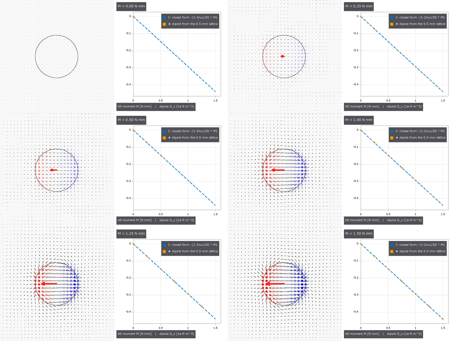
↑ The measurement ―― 傾きモーメントを 0 → 1.5 N·mm に 7 段で上げる。左 = マーカー 1 個ごとの発散(赤 +・青 −、押し込み子の縁に正負の対が立つ)と変位(60 倍)、赤矢印 = 双極子(長さ ∝ M)。右 = 格子マーカーの双極子 D_x が閉形式の線 −(1−2ν)/2G·M1(破線)に乗る: R² = 1.000000、傾きの比 0.9997。 (figure labels are in Japanese; the numbers are the same)

↑ 重ね合わせた場(傾き 1 N·mm + ねじり 0.5 N·mm + 並進 1 px)を 3 つに分ける: 発散の双極子が傾き(M1 = 1.015 N·mm、真値 0.991、窓 a + 当てはめ半径)、剛体回転の最小二乗がねじり(M_z = 0.497 N·mm、真値 0.500、窓 0.9a)…

↑ 第 2 真値: 有限要素の節点変位(有限厚のドーム状ゲル、Robo-Touch/Taxim リポジトリ同梱、MIT、節点 15,230・間隔 0.155 mm)。

↑ 壊れる場所。

↑ 圧力の 1 次モーメントが同じ 1 N·mm の 3 つの押し込み子: 平頭にモーメント、Hertz 球を M/P だけずらす、細長い楕円(稜)をずらす。
py -3.11 examples/poc_tactile_dipole_torque.py
Source: examples/poc_tactile_dipole_torque.py
This run produced 6 figures in total - see them all
Ops used (notes): boussinesq_kernel · boussinesq_surface_displacement · cerruti_kernel · combined_modulus · dipole_to_torque_fit · dipole_torque_resolution · displace_markers · ellipse_pressure_shifted · fem_nodes_load · grasp_torque_frame · hertz_pressure · hertz_pressure_shifted · hertz_sphere · hertz_surface_ur · hertz_surface_uz · marker_divergence · marker_image · membrane_lights · membrane_markers · membrane_render_markers · membrane_render_rgb · membrane_shear_field · mindlin_partial_slip · pad_context … (+12)
No.2026.202 —— Measuring a Powder Heap from Images — Angle of Repose, Volume, Mass, Flowability and Discharge by Rules, with Closed Forms, Published Values and MuJoCo as the Truth
The physics-simulation × Fullseye series continues (after pegsim, tacsim, tacslip, tactorque, puck and pegfail). The prior work on powder weighing (Kadokawa, Hamaya, Tanaka, IROS 2023, doi 10.1109/iros55552.2023.10342463) observes only the scale reading and has no vision. This exhibit fills in the other side — reading the angle of repose, volume, mass, flowability and discharge rate from the shape of the heap (a side image and a heightmap) — with the new module granular (23 ops plus 2 mujoco facades), learning-free. Ground truth comes from outside on four fronts. (1) Closed forms: the cone V = (π/3)R²H, H = R tan φ, m = ρ_b V; the Beverloo, Leniger and van de Velde (1961) discharge law W = C ρ_b √g (D₀ − k d)^{5/2} (C ≈ 0.58, k ≈ 1.4 as summarised by Nedderman 1992). (2) A published table: Table 1 of USP general chapter <1174> Powder Flow (angle of repose → flow property, after Carr 1965) — the table is in whole degrees, so the angle is rounded first (30.4 → excellent, 30.5 → good, below 25 is outside the table). (3) A published value: 25.2 ± 0.8 degrees for 1 mm glass beads (Sunday, Murdoch, Tardivel, Schwartz, Michel, MNRAS 2020, arXiv 2009.10448 §5.4); the way of measuring (separate lines on the left and right upper edges of a side image, tails and apex excluded, §5.3) is taken from the same paper. (4) A second implementation (–full): 1,200 rigid spheres in MuJoCo 3 (r 4 mm, sliding friction 0.16, rolling 0.09·R) flow out of a square orifice (48 mm) in a flat-bottomed hopper and build a heap. The side-image measurement reads the coverage of the edge pixel directly as a sub-pixel position (edge method): with uniform noise ±0.1 on the coverage it stays within 0.0064 degrees. ★The column-sum method (summed coverage = powder height) shrinks tan φ by the ratio 0.975 that clipping the noise to [0, 1] leaves in the powder pixels, and reads −0.63 degrees low — at first misread as a toe-rounding bias, until it survived with no rounding at all. The heightmap path takes the mode of the demops.dem_slope histogram (noise only ever raises the gradient: +0.12 degrees at σ 0.05 px, +0.37 at 0.1 px). ★A tilted datum β = 5 degrees adds to the angle of repose: the flanks read 33.62 / 26.10 degrees = the closed form atan(tan φ ± tan β), the 7.52-degree left-right difference raises the alarm (datum_tilt_check), and subtracting tangents brings back 30.0000. The heightmap mode reads 5.00 degrees — the ground itself, because the ground cells take over the histogram (29.9994 once the datum is passed). A sheared datum and a camera roll differ to first order on one flank (33.62 vs 35.00), so the two corrections must not be confused. Figures: the two lines fitted to a side image (1:1), the slope histogram, where resolution breaks it (heap widths 25–400 px), toe rounding, apex blunting, the tilted datum and a 50 px heap (×10, pixels visible), Beverloo’s W(D₀), the flowability bands with the published and MuJoCo values, the spoon tilt, and a GIF sweeping the datum tilt from −8 to +8 degrees; with –full: a GIF of the spheres flowing out of the orifice into a heap (bin walls and floor drawn), the lines fitted to the sphere heap’s side with the published 25.2-degree slope, the heightmap, the discharged mass against Beverloo’s slope, and a table of MuJoCo vs the outside references. 20 gates (numpy, 1.3 s) plus 5 with –full (MuJoCo, 34 s): cone round trips 1.8e-16, heightmap volume 3.5e-7, side-image round trip 0.0000 degrees, Beverloo exponent n = 2.5074 and C = 0.5894 from six synthetic discharge heightmap videos with σ 0.5 mm (noiseless n = 2.5000000), W(30 mm, 1 mm, 1500) = 0.3769 kg/s, toe rounding −0.248 → −0.001 degrees with 15 % of the toe excluded, apex blunting −0.554 → −0.004, resolution (noise ±0.1, 4 angles × 6 seeds: 0.197 degrees for a 50 px heap and 0.624 for 25 px from the side, 1.097 for 50 px from the heightmap), 16 flowability boundaries, ValueError for spelling breaks and for heaps that are absent or cut off, the spoon rule θ_c = φ − atan(2h₀/L) (our own derivation: 18.69 degrees at L 50 mm, h₀ 5 mm; φ as h₀ → 0. On 2026-10-05 the wedge slope was corrected from the small-angle tan φ − tan θ (20.67 degrees then) to the exact tan(φ − θ), and a container with no lip wall, which spills from θ = 0⁺, was added), container fill 0.6300 with a 3.000-degree surface, mass from video (the same cone on both sides, so it checks the plumbing only), the MJCF string and the entry points; –full: the heap formed (0 runaways, 114 left in the stagnant layer of the bin, 38.4 mm tall = 4.8 diameters), the mean of four azimuths (22.4 / 23.0 / 18.9 / 24.4) 22.17 degrees vs the published 25.2 ± 0.8 → −3.03 (gate −7 to +1), the median of the heightmap smoothed over two diameters 25.74 degrees (the unsmoothed mode 65.5 = sphere rims), discharge 0.906 kg/s vs Beverloo 0.911 kg/s (square orifice as an equivalent diameter of 54.2 mm, ρ_b 1312 kg/m³ measured in the bin). Honestly: the synthetic side image shares its edge model with the measurement, so the noiseless round trip checks the plumbing; the only independent subjects are the noise and MuJoCo’s spheres. Why the MuJoCo heap sits 3 degrees below the published value (rigid soft contact without cohesion, a rolling-friction model unlike DEM, a heap only five diameters tall, 18.9–24.4 degrees by azimuth from the square orifice’s flow) is not resolved. The 0.99 ratio to Beverloo agrees too well to be trusted and is kept as an order-of-magnitude gate (1.02 and 1.14 in earlier configurations; D₀/d = 6.8 is near the jamming limit; 14 frames in the band). The per-material table of Al-Hashemi & Al-Amoudi 2018 (CC BY 4.0) could not be retrieved and is not included; the empirical formula of Zhou et al. 2002 was not read. Milligram weighing is beyond the volume resolution of an image (it works for gram-scale gravel and beads; milligrams belong to the scale). Container fill assumes the image is the inner wall (wall detection is not implemented). Traps we hit: on a smooth floor (μ 0.16) the 1,200 spheres spread into a single layer 0.15 m in radius and no heap formed — a single-sphere test showed rolling resistance saturates at the sliding limit μ_s g (1.6 m/s² for rolling coefficients of both 0.01 and 0.1), so the floor was made rough with μ 1.0 (as experiments glue sandpaper to the base); a soft-contact time constant below 2·timestep diverges (the op refuses it); the Newton solver stalls on a dense heap beyond 280 s → CG with an elliptic cone.

↑ Measuring a Powder Heap from Images — Angle of Repose, Volume, Mass, Flowability and Discharge by Rules, with Closed Forms, Published Values and MuJoCo as the Truth ―― The physics-simulation × Fullseye series continues (after pegsim, tacsim, tacslip, tactorque, puck and pegfail). The prior work on powder weighing (Kadokawa, Hamaya, Tanaka, IROS 2023, doi 10.1109/iros55552.2023.10342463) observes only the scale reading and has no vision. This exhibit fills in the other side — reading the angle of repose, volume, mass, flowability and discharge rate from the shape of the heap (a side image and a heightmap) — with the new module granular (23 ops plus 2 mujoco facades), learning-free. Ground truth comes from outside on four fronts. (1) Closed forms: the cone V = (π/3)R²H, H = R tan φ, m = ρ_b V; the Beverloo, Leniger and van de Velde (1961) discharge law W = C ρ_b √g (D₀ − k d)^{5/2} (C ≈ 0.58, k ≈ 1.4 as summarised by Nedderman 1992). (2) A published table: Table 1 of USP general chapter <1174> Powder Flow (angle of repose → flow property, after Carr 1965) — the table is in whole degrees, so the angle is rounded first (30.4 → excellent, 30.5 → good, below 25 is outside the table). (3) A published value: 25.2 ± 0.8 degrees for 1 mm glass beads (Sunday, Murdoch, Tardivel, Schwartz, Michel, MNRAS 2020, arXiv 2009.10448 §5.4); the way of measuring (separate lines on the left and right upper edges of a side image, tails and apex excluded, §5.3) is taken from the same paper. (4) A second implementation (–full): 1,200 rigid spheres in MuJoCo 3 (r 4 mm, sliding friction 0.16, rolling 0.09·R) flow out of a square orifice (48 mm) in a flat-bottomed hopper and build a heap. The side-image measurement reads the coverage of the edge pixel directly as a sub-pixel position (edge method): with uniform noise ±0.1 on the coverage it stays within 0.0064 degrees. ★The column-sum method (summed coverage = powder height) shrinks tan φ by the ratio 0.975 that clipping the noise to [0, 1] leaves in the powder pixels, and reads −0.63 degrees low — at first misread as a toe-rounding bias, until it survived with no rounding at all. The heightmap path takes the mode of the demops.dem_slope histogram (noise only ever raises the gradient: +0.12 degrees at σ 0.05 px, +0.37 at 0.1 px). ★A tilted datum β = 5 degrees adds to the angle of repose: the flanks read 33.62 / 26.10 degrees = the closed form atan(tan φ ± tan β), the 7.52-degree left-right difference raises the alarm (datum_tilt_check), and subtracting tangents brings back 30.0000. The heightmap mode reads 5.00 degrees — the ground itself, because the ground cells take over the histogram (29.9994 once the datum is passed). A sheared datum and a camera roll differ to first order on one flank (33.62 vs 35.00), so the two corrections must not be confused. Figures: the two lines fitted to a side image (1:1), the slope histogram, where resolution breaks it (heap widths 25–400 px), toe rounding, apex blunting, the tilted datum and a 50 px heap (×10, pixels visible), Beverloo’s W(D₀), the flowability bands with the published and MuJoCo values, the spoon tilt, and a GIF sweeping the datum tilt from −8 to +8 degrees; with –full: a GIF of the spheres flowing out of the orifice into a heap (bin walls and floor drawn), the lines fitted to the sphere heap’s side with the published 25.2-degree slope, the heightmap, the discharged mass against Beverloo’s slope, and a table of MuJoCo vs the outside references. 20 gates (numpy, 1.3 s) plus 5 with –full (MuJoCo, 34 s): cone round trips 1.8e-16, heightmap volume 3.5e-7, side-image round trip 0.0000 degrees, Beverloo exponent n = 2.5074 and C = 0.5894 from six synthetic discharge heightmap videos with σ 0.5 mm (noiseless n = 2.5000000), W(30 mm, 1 mm, 1500) = 0.3769 kg/s, toe rounding −0.248 → −0.001 degrees with 15 % of the toe excluded, apex blunting −0.554 → −0.004, resolution (noise ±0.1, 4 angles × 6 seeds: 0.197 degrees for a 50 px heap and 0.624 for 25 px from the side, 1.097 for 50 px from the heightmap), 16 flowability boundaries, ValueError for spelling breaks and for heaps that are absent or cut off, the spoon rule θ_c = φ − atan(2h₀/L) (our own derivation: 18.69 degrees at L 50 mm, h₀ 5 mm; φ as h₀ → 0. On 2026-10-05 the wedge slope was corrected from the small-angle tan φ − tan θ (20.67 degrees then) to the exact tan(φ − θ), and a container with no lip wall, which spills from θ = 0⁺, was added), container fill 0.6300 with a 3.000-degree surface, mass from video (the same cone on both sides, so it checks the plumbing only), the MJCF string and the entry points; –full: the heap formed (0 runaways, 114 left in the stagnant layer of the bin, 38.4 mm tall = 4.8 diameters), the mean of four azimuths (22.4 / 23.0 / 18.9 / 24.4) 22.17 degrees vs the published 25.2 ± 0.8 → −3.03 (gate −7 to +1), the median of the heightmap smoothed over two diameters 25.74 degrees (the unsmoothed mode 65.5 = sphere rims), discharge 0.906 kg/s vs Beverloo 0.911 kg/s (square orifice as an equivalent diameter of 54.2 mm, ρ_b 1312 kg/m³ measured in the bin). Honestly: the synthetic side image shares its edge model with the measurement, so the noiseless round trip checks the plumbing; the only independent subjects are the noise and MuJoCo’s spheres. Why the MuJoCo heap sits 3 degrees below the published value (rigid soft contact without cohesion, a rolling-friction model unlike DEM, a heap only five diameters tall, 18.9–24.4 degrees by azimuth from the square orifice’s flow) is not resolved. The 0.99 ratio to Beverloo agrees too well to be trusted and is kept as an order-of-magnitude gate (1.02 and 1.14 in earlier configurations; D₀/d = 6.8 is near the jamming limit; 14 frames in the band). The per-material table of Al-Hashemi & Al-Amoudi 2018 (CC BY 4.0) could not be retrieved and is not included; the empirical formula of Zhou et al. 2002 was not read. Milligram weighing is beyond the volume resolution of an image (it works for gram-scale gravel and beads; milligrams belong to the scale). Container fill assumes the image is the inner wall (wall detection is not implemented). Traps we hit: on a smooth floor (μ 0.16) the 1,200 spheres spread into a single layer 0.15 m in radius and no heap formed — a single-sphere test showed rolling resistance saturates at the sliding limit μ_s g (1.6 m/s² for rolling coefficients of both 0.01 and 0.1), so the floor was made rough with μ 1.0 (as experiments glue sandpaper to the base); a soft-contact time constant below 2·timestep diverges (the op refuses it); the Newton solver stalls on a dense heap beyond 280 s → CG with an elliptic cone.
| [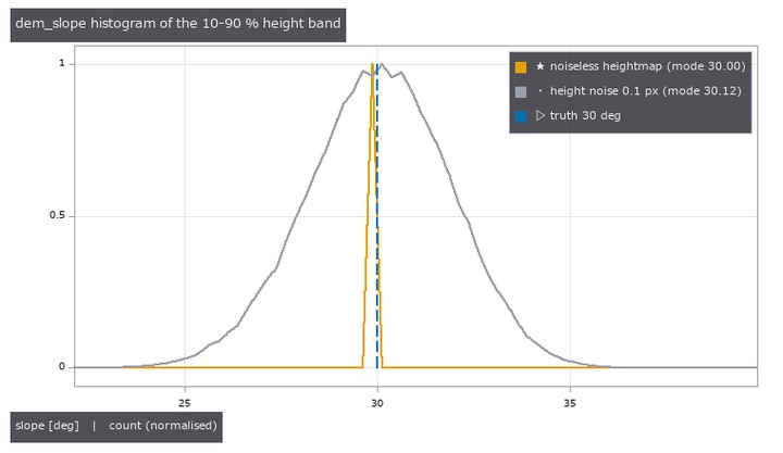](https://raw.githubusercontent.com/furuse-kazufumi/fullseye/master/docs/articles/assets/poc/poc_granular_heap_repose/02_granular_slope_histogram.png) |
| *↑ The measurement ―― 高さ図の勾配ヒストグラム(demops.dem_slope)。雑音なしは 1 ビンに立つ。σ = 0.1 px の雑音で最頻が +0.12 度ずれる( | ∇ | は雑音で増えるだけ)—— 同じ大きさの雑音で側面像は 0.01 度も動かない。 (figure labels are in Japanese; the numbers are the same)* |

↑ 山の幅(画素)と φ の最大誤差(2 角度 × 8 seed)。

↑ 基準面が 5 度傾くと左右が 33.62 / 26.10 度に割れる(atan(tan φ ± tan β))。

↑ 安息角 → 流動性区分(USP <1174> 表 1、原典 Carr 1965)。

↑ 同じ山の高さ図(単位 mm、球面の最大高さ、1.5 mm/セルを 3 倍の最近傍で表示)。
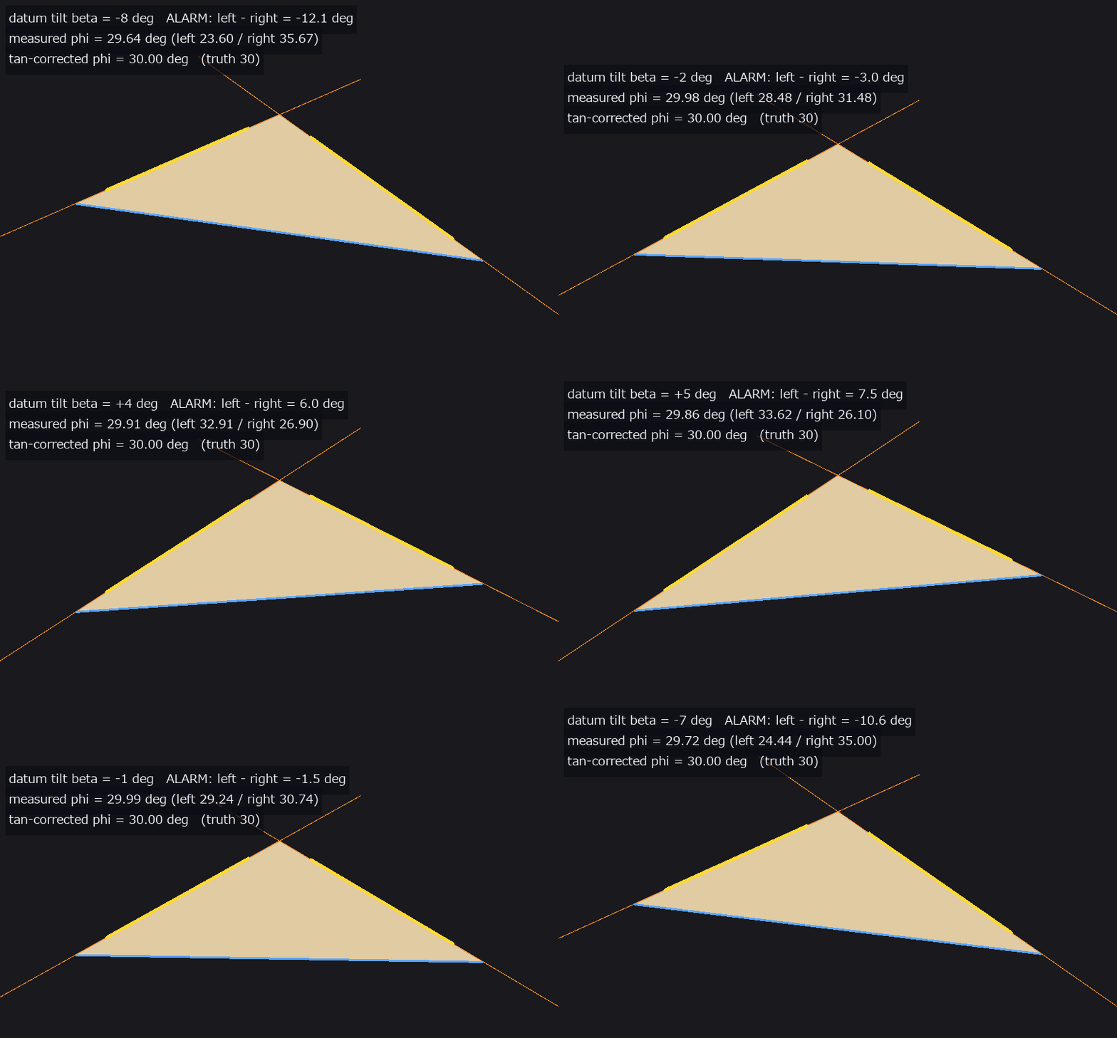
↑ The animation ―― 基準面の傾き β を −8〜+8 度で振る(32 コマ)。左右の斜面が atan(tan φ ± tan β) で割れ、左右差 ≈ 2β が 1 度を超えると警報。tan の引き算で 30 度に戻る。
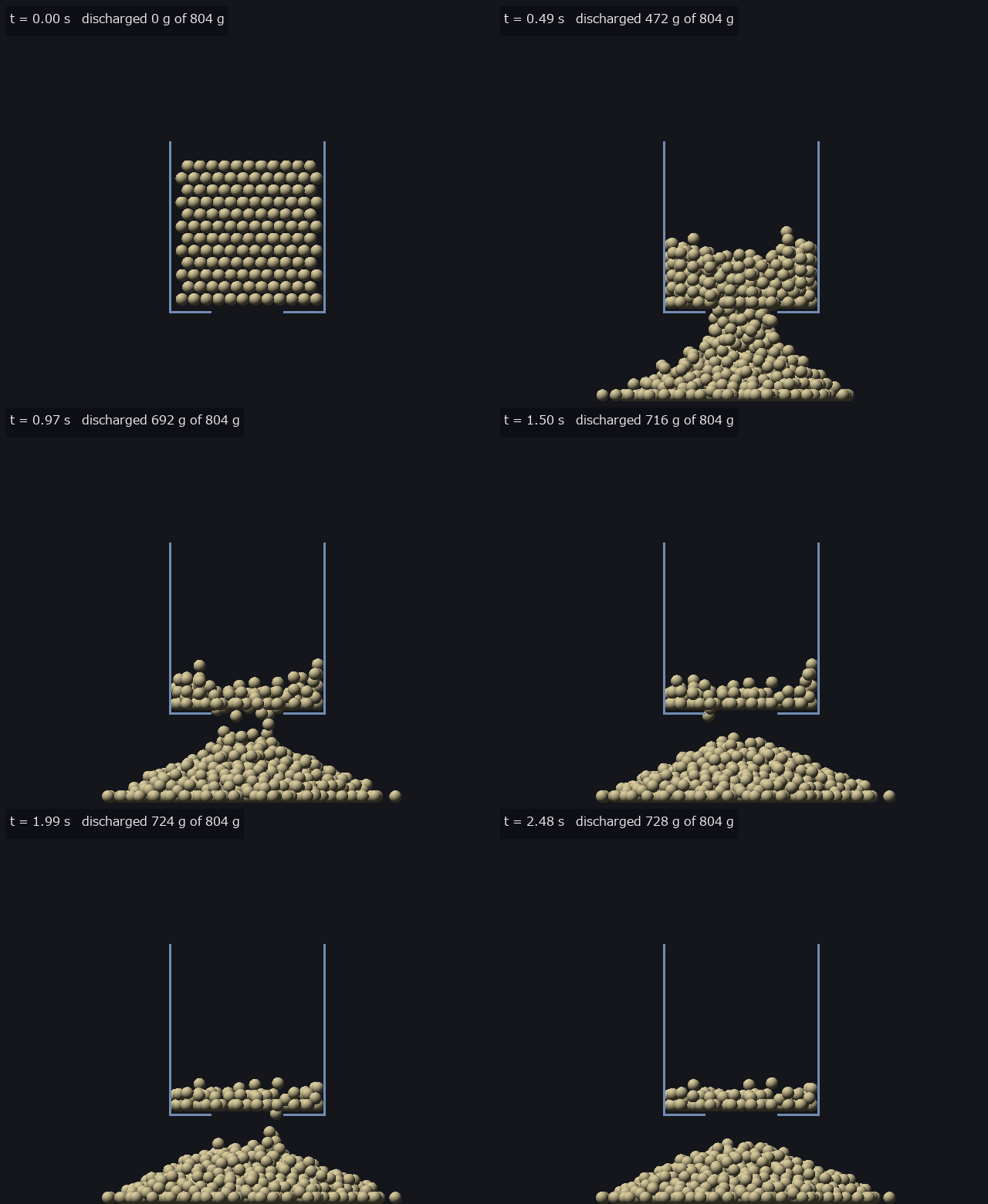
↑ The animation ―― 剛体球 1200 個(r 4 mm、滑り摩擦 0.16、転がり 0.09·R、粗い台)が平底ホッパ(青灰の線 = 壁と底板)の正方孔(48 mm)から流れて山になる(0.5 mm/px、67 コマ)。φ = 22.17 度(4 方位の平均)。
py -3.11 examples/poc_granular_heap_repose.py
Source: examples/poc_granular_heap_repose.py
This run produced 16 figures in total - see them all
Ops used (notes): beverloo_fit · beverloo_rate · container_fill_level · container_synth · datum_tilt_check · difference · discharge_synth · dispense_mass_from_video · heap_mass · heap_scene_mjcf · heap_spheres_select · heap_synth_cone · heap_volume_cone · heap_volume_heightmap · hopper_discharge_rate · powder_flowability_class · repose_angle_heightmap · repose_angle_silhouette · spheres_render_shaded · spheres_to_heightmap · spheres_to_silhouette · spoon_tilt_critical · spoon_tilt_dispense · text_box
No.2026.205 —— Measuring Food Cutting from Images — Knife Tracking, Slice Thickness, Cut-Surface Roughness and Cutting Force from Wrist Deflection, with Closed Forms and MuJoCo as the Truth
The physics-simulation × Fullseye series. The subject is robotic food slicing (arXiv:2404.02569, ICRA 2024). Without learning, rules alone close the chain image → knife height → soft-wrist deflection → force → toughness R. New module cutting, 16 ops plus 1 mujoco facade. Ground truth comes from outside on three fronts. (1) Closed-form cutting mechanics: equations 1.1–1.4 of Atkins, Interface Focus 6:20160019 (2016) (frictionless push + slice, V/(Rw) = 1/(1+ξ²), H = ξV, F_res/(Rw) = 1/√(1+ξ²)) with the numbers in the text (H/Rw peaks at 0.5 at ξ = 1; a tilted blade moved vertically gives ξ = tan i), and equation 2.6 of Williams & Patel, Interface Focus 6:20150108 (2016) (wedge + Coulomb friction, minimum 1/(1 − sin β)) with the worked example (μ = 0.2 gives θo = 79° and a minimum of 1.24). The slice/push equations with friction and blade angle were not read, so they are not implemented and the combination raises ValueError. (2) The physics engine MuJoCo (–full): the blade rendered by an orthographic camera is followed by the same tracker and compared with the wrist constraint force, where the food resistance is replaced each step by a joint friction loss R·w_eff·g(ξ). A soft body matches the stiffness order of magnitude but does not fracture (the blade sinks in), and a gate pins that. (3) Finite-element blade forces (–full, optional, non-commercial): the CSV published with arXiv:2105.12244 (CC BY-NC 4.0) is read from an environment variable and compared by shape only (the data is not in the repo and not in the figures). ★Slice-thickness edges are read by unmixing each row into three colours (background, food, blade): the background fraction steps 1 → 0 at the end face and the blade fraction 0 → 1 at the blade face, so the sum inside a window is the edge position. Blur does not change the sum, so widening the window from the step’s second moment removes the bias — the thickness bias at 4 px blur goes from −18 µm to +11 µm, and 8 px is refused because the blade band is too thin for the blur (the prototype passed silently at −37 µm). ★For a thin slice the reference food colour comes from the body beyond the blade, so a left-right illumination gradient shifts it by 13 %: estimating the illumination from the blade band’s brightness and correcting brings 66 µm down to 5 µm. Figures: a GIF of a synthetic cut (estimated edge line, dashed where hidden, truth, tip and the force curve), the edge-on image with both edges, the thickness distribution and scatter over 40 images, the cut-surface profile, where it breaks, the slice/push closed form; with –full: a MuJoCo GIF and the force of a blade pressed into a soft body. 14 gates (numpy, CPU 0.95 s) plus 7 with –full: closed forms 1e-16, H/Rw maximum 0.5000 at ξ 1.000, θo 78.69° and minimum 1.2440, angle 0.017°, hidden mid-span edge 8.2 µm, tip 0.24 mm, depth 29 µm (0.12 px), thickness 0.1–5 mm with bias 6.9 µm and per-row RMS 18.5 µm, tilt 0.021°, roughness floor Rq 11 µm, R 393.6 (truth 400, −1.6 %) and ξ 0.561 (truth 0.570), R 500.0 in a world with 1.25× force (self-reported); –full (8 px/mm and 20 px/mm): angle 0.0014°, edge 1.1 µm, depth 2.2 µm, thickness bias 2.8 µm and RMS 10.4 µm, ≤ 5 µm up to noise 0.05 with 0.1 refused, MuJoCo soft body F/(E·A·δ/H) 1.106 / 1.074 / 1.059, the blade saturating at 0.76 N, render → track 0.9 µm and 0.0007°, wrist force 0.083 N ≤ c·v 0.150 N, FEM residual / steady value ≤ 0.068 over 6 curves. Honestly: no force truth comes from outside — the synthetic forces and the fit use the same Atkins model, so the image → R chain checks the plumbing (in a world with 1.25× force, R simply comes out 1.25× and toughness cannot be separated from friction). The food is assumed not to deform, the blade edge straight and single-bevelled. No measured toughness values are quoted. No public cutting dataset with images was found. The MuJoCo soft body keeps oscillating by ±5–11 % while held. Traps we hit: the image centre is ((H−1)/2, (W−1)/2) (H/2 shifts it by 62.5 µm), MuJoCo’s friction loss is viscous-soft by default, and estimating ξ from the entry part of the trajectory gives 0.63 (truth 0.57).
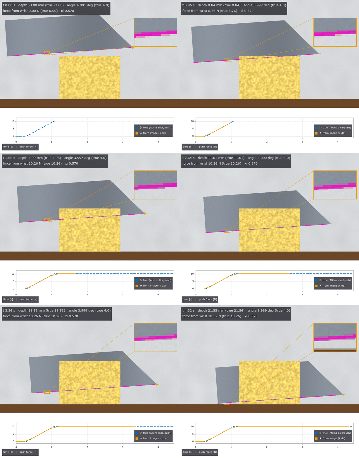
↑ Measuring Food Cutting from Images — Knife Tracking, Slice Thickness, Cut-Surface Roughness and Cutting Force from Wrist Deflection, with Closed Forms and MuJoCo as the Truth ―― The physics-simulation × Fullseye series. The subject is robotic food slicing (arXiv:2404.02569, ICRA 2024). Without learning, rules alone close the chain image → knife height → soft-wrist deflection → force → toughness R. New module cutting, 16 ops plus 1 mujoco facade. Ground truth comes from outside on three fronts. (1) Closed-form cutting mechanics: equations 1.1–1.4 of Atkins, Interface Focus 6:20160019 (2016) (frictionless push + slice, V/(Rw) = 1/(1+ξ²), H = ξV, F_res/(Rw) = 1/√(1+ξ²)) with the numbers in the text (H/Rw peaks at 0.5 at ξ = 1; a tilted blade moved vertically gives ξ = tan i), and equation 2.6 of Williams & Patel, Interface Focus 6:20150108 (2016) (wedge + Coulomb friction, minimum 1/(1 − sin β)) with the worked example (μ = 0.2 gives θo = 79° and a minimum of 1.24). The slice/push equations with friction and blade angle were not read, so they are not implemented and the combination raises ValueError. (2) The physics engine MuJoCo (–full): the blade rendered by an orthographic camera is followed by the same tracker and compared with the wrist constraint force, where the food resistance is replaced each step by a joint friction loss R·w_eff·g(ξ). A soft body matches the stiffness order of magnitude but does not fracture (the blade sinks in), and a gate pins that. (3) Finite-element blade forces (–full, optional, non-commercial): the CSV published with arXiv:2105.12244 (CC BY-NC 4.0) is read from an environment variable and compared by shape only (the data is not in the repo and not in the figures). ★Slice-thickness edges are read by unmixing each row into three colours (background, food, blade): the background fraction steps 1 → 0 at the end face and the blade fraction 0 → 1 at the blade face, so the sum inside a window is the edge position. Blur does not change the sum, so widening the window from the step’s second moment removes the bias — the thickness bias at 4 px blur goes from −18 µm to +11 µm, and 8 px is refused because the blade band is too thin for the blur (the prototype passed silently at −37 µm). ★For a thin slice the reference food colour comes from the body beyond the blade, so a left-right illumination gradient shifts it by 13 %: estimating the illumination from the blade band’s brightness and correcting brings 66 µm down to 5 µm. Figures: a GIF of a synthetic cut (estimated edge line, dashed where hidden, truth, tip and the force curve), the edge-on image with both edges, the thickness distribution and scatter over 40 images, the cut-surface profile, where it breaks, the slice/push closed form; with –full: a MuJoCo GIF and the force of a blade pressed into a soft body. 14 gates (numpy, CPU 0.95 s) plus 7 with –full: closed forms 1e-16, H/Rw maximum 0.5000 at ξ 1.000, θo 78.69° and minimum 1.2440, angle 0.017°, hidden mid-span edge 8.2 µm, tip 0.24 mm, depth 29 µm (0.12 px), thickness 0.1–5 mm with bias 6.9 µm and per-row RMS 18.5 µm, tilt 0.021°, roughness floor Rq 11 µm, R 393.6 (truth 400, −1.6 %) and ξ 0.561 (truth 0.570), R 500.0 in a world with 1.25× force (self-reported); –full (8 px/mm and 20 px/mm): angle 0.0014°, edge 1.1 µm, depth 2.2 µm, thickness bias 2.8 µm and RMS 10.4 µm, ≤ 5 µm up to noise 0.05 with 0.1 refused, MuJoCo soft body F/(E·A·δ/H) 1.106 / 1.074 / 1.059, the blade saturating at 0.76 N, render → track 0.9 µm and 0.0007°, wrist force 0.083 N ≤ c·v 0.150 N, FEM residual / steady value ≤ 0.068 over 6 curves. Honestly: no force truth comes from outside — the synthetic forces and the fit use the same Atkins model, so the image → R chain checks the plumbing (in a world with 1.25× force, R simply comes out 1.25× and toughness cannot be separated from friction). The food is assumed not to deform, the blade edge straight and single-bevelled. No measured toughness values are quoted. No public cutting dataset with images was found. The MuJoCo soft body keeps oscillating by ±5–11 % while held. Traps we hit: the image centre is ((H−1)/2, (W−1)/2) (H/2 shifts it by 62.5 µm), MuJoCo’s friction loss is viscous-soft by default, and estimating ξ from the entry part of the trajectory gives 0.63 (truth 0.57).

↑ The measurement ―― 刃先方向の像(20 px/mm、等倍): 片刃の平らな面と食材の端面の距離 = 切片の厚み。破線 = 推定の両縁。 (figure labels are in Japanese; the numbers are the same)
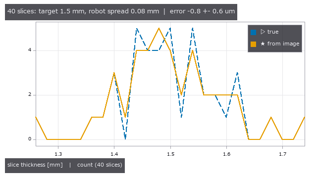
↑ 狙い 1.5 mm・ばらつき σ 0.08 mm・傾き σ 0.5° の 40 枚: 真値(破線)と画像(実線)の分布。
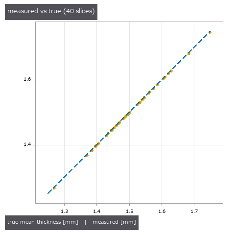
↑ 40 枚の測った厚み vs 真値(破線 = y = x)。

↑ 雑音とぼけを強めたときの深さ・厚みの誤差(元の解像度)。

↑ 摩擦なしの slice/push の閉形式。
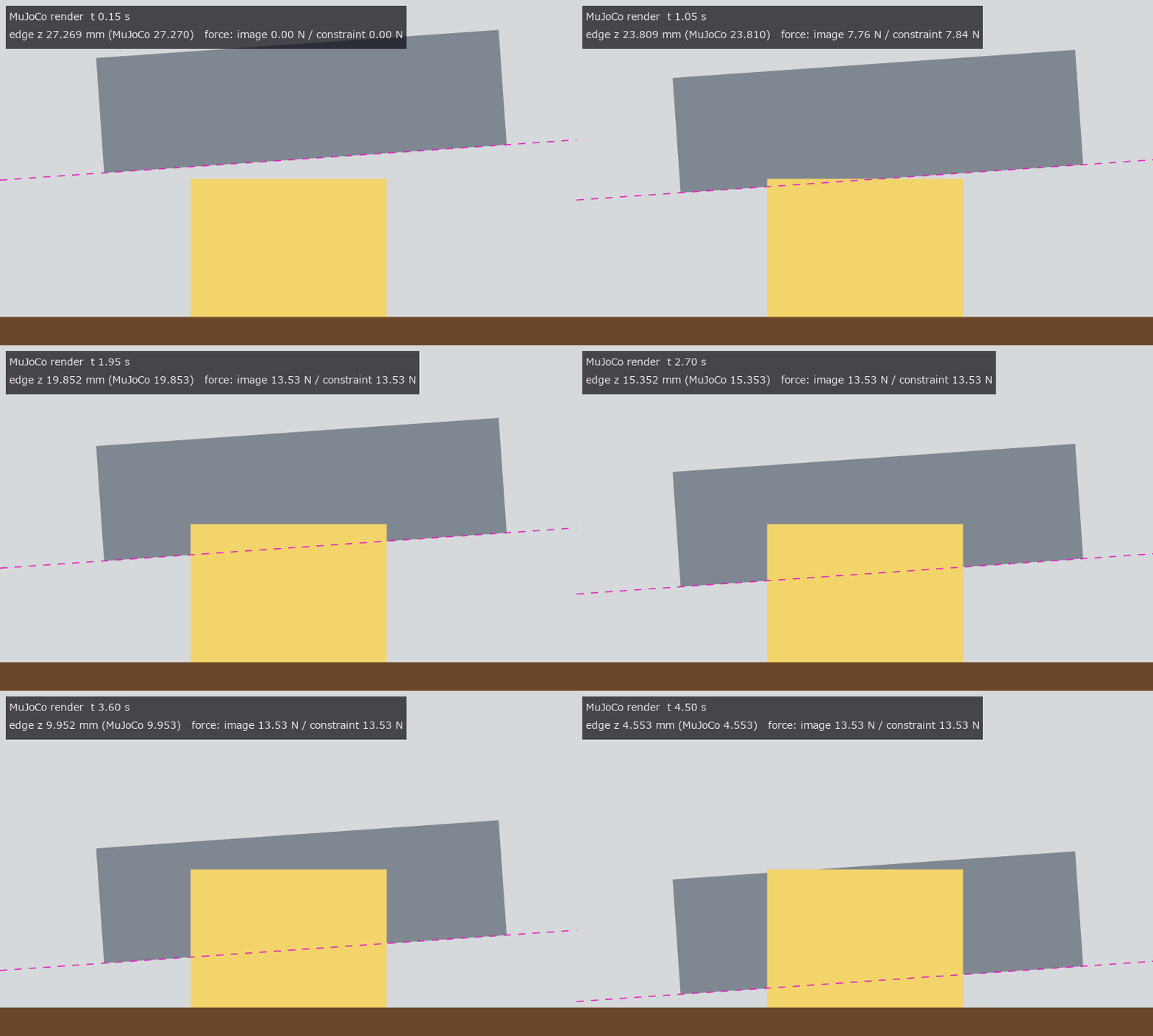
↑ The animation ―― MuJoCo の正射影カメラで描いた刃(柔らかい手首 4 N/mm、抵抗 = 摩擦損失 = Atkins の切断力)を同じ追跡器で追う。破線 = 推定の刃先線。
py -3.11 examples/poc_food_cutting_measure.py
Source: examples/poc_food_cutting_measure.py
This run produced 9 figures in total - see them all
Ops used (notes): cut_depth_from_side · cut_force_atkins · cut_force_csv_load · cut_force_fit · cut_surface_roughness · cutting_edge_render · cutting_episode_synth · cutting_face_render · cutting_scene · cutting_wrist_mjcf · food_cut_width · force_from_wrist_displacement · identity · knife_edge_track · profile_params · slice_push_from_track · slice_push_ratio · slice_thickness_profile · text_box · zoom_inset
No.2026.207 —— Gating Large-Deformation Contact of a Soft Dome Fingertip Pressed on a Flat Object with a Scaling Law and an Exact Continuum Solution — As Printed, the Linear Coefficient of Eq. (3) Makes the Force of a Cylinder Negative; 2n/(1+n) Is Derived from the Paper’s Own Model
The physics-simulation × Fullseye series (vision-based touch), the next step beyond tacsim (a Hertz membrane, small strain). The primary source is the PDF of T. Mu et al., “A scaling law for large-deformation contact in soft materials” (arXiv:2509.18581, 2025). It is set up as a soft dome fingertip sensor (a hemisphere, height L = radius R = 8 mm, μ = 0.1 MPa as design assumptions) pressed onto a flat object. The framework: the linear solution F_L = C δⁿ for a profile f = c rᵖ (n = 1 + 1/p), large deformation F = κₙ(δ/L) F_L, the contact radius of eq. (4) (incomplete beta) and the universal form κ = (1 − 10/9·δ/L)⁻¹. New module tacdome, 12 ops, all numpy. ★The linear coefficient of eq. (3): the print, read from a 400 dpi image of the page, says (4+2n)/(1+n), which gives κ₁(0.5) = −1.667 for a cylinder (a negative force). Integrating the paper’s own model (a neo-Hookean cylindrical spring of length L − g at every point of the 1-D profile) gives c₁ = 2n/(1+n) and c₂ = n/(2+n), and a contact radius identical to eq. (4) — the quadratic term and eq. (4) agree with the print; only the linear term differs. A variant with all springs of length L gives (1.008, 0.258), matching neither reading. The appendix is not on arXiv and was not read. Ground truth from outside on three fronts: the exact uniaxial compression of an incompressible neo-Hookean cylinder (1.9e-15 from the derived κ₁), the small-strain Hertz limit (1e-12 from tacsim, the subject), and the paper’s universal k = 10/9 (least squares of the derived κ₁⁻¹ gives 1.1060, 0.5 % off). Second implementation = midpoint rule over the spring bed (8.5e-9 from the closed form); three routes to eq. (4) agree to 1e-15. The derived κ⁻¹(0.5) = 0.429 / 0.493 / 0.545 (n = 1 / 1.5 / 2) has the same order as the inset of the paper’s Fig. 4B. The subject’s result — how wrong it is depends on what you observe: for a hemispherical fingertip, Hertz force read from indentation is −4.10 / −27.79 / −50.70 % at δ/L = 0.05 / 0.3 / 0.5 and the radius −1.71 / −11.70 / −22.20 %. But reading force from the contact radius with Hertz (how a vision-based tactile sensor reads it), κ and the radius growth nearly cancel: max +5.39 % (d = 0.4). A cone does not cancel (−18.95 % at d = 0.5); a flat punch cannot be read, since its radius does not fix δ. From the internal camera image (192 px, 0.117 mm/px) the area method (a linear sum of unclipped coverage) gives the radius within 0.004 %, the inverted force within 0.013 % and 0.411 % with noise σ = 0.03; fitting measure.fit_circle to edge pixels gives −0.61 to −2.51 %. With –full: 0.0049 % radius and 0.0146 % force over 20 points at 512 px; a MuJoCo soft body (a linear-elastic cube compressed without friction) matches only the linear limit (stiffness ratio 0.98–0.99 at small strain) and collapses to 0.18 at ε = 0.31 — useless as a large-deformation truth (gated at small strain only). Figures: a GIF of the press (internal camera image, spring bed, force curve), force for three shapes, the κ⁻¹ band and three readings, a/a_L with the exact cylinder, the Hertz error, a 24× crop of the contact edge; with –full: the soft-body stiffness ratio. 13 gates (default, 0.2 s) plus 2 with –full (41 s with figures). Honestly: Fig. 5C (radius vs force) is not reproduced (the derived model differs by 0–1.7 % in radius at equal force; the sensor dimensions in the appendix were not read). Nor is “all shapes fall in a narrow band described by the universal form” (the universal form is 10.9 % above the sphere and 22.7 % above the cone). The cylinder experiments include friction and are not gated. The hemisphere is approximated by a paraboloid; frictionless, quasi-static, incompressible; idealised lighting. Trap we hit: the figure captions printed the pixel pitch in metres labelled as mm (0.000 mm/px), fixed on inspection during integration.
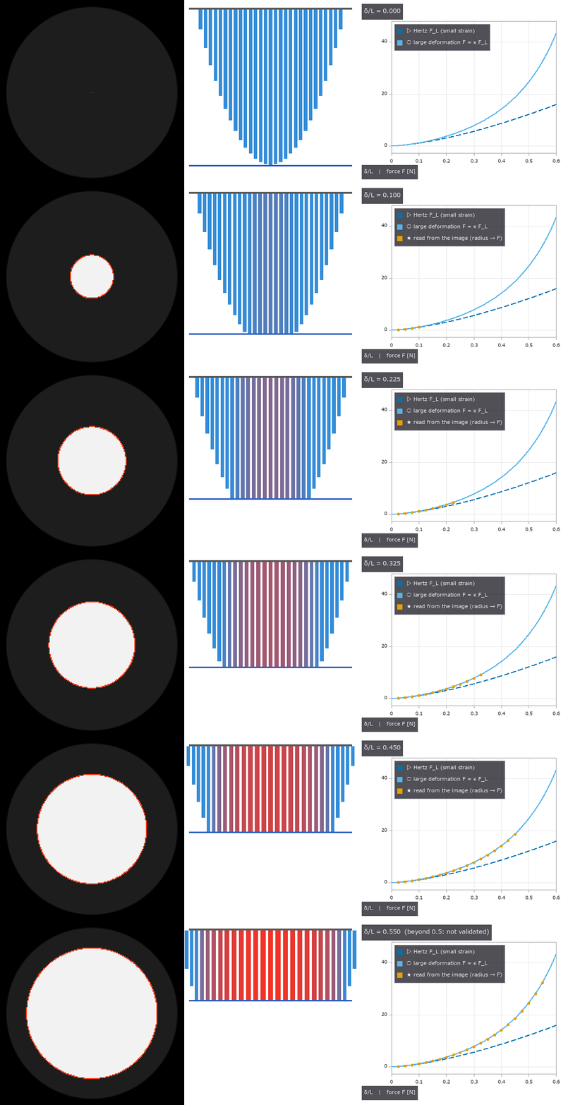
↑ Gating Large-Deformation Contact of a Soft Dome Fingertip Pressed on a Flat Object with a Scaling Law and an Exact Continuum Solution — As Printed, the Linear Coefficient of Eq. (3) Makes the Force of a Cylinder Negative; 2n/(1+n) Is Derived from the Paper’s Own Model ―― The physics-simulation × Fullseye series (vision-based touch), the next step beyond tacsim (a Hertz membrane, small strain). The primary source is the PDF of T. Mu et al., “A scaling law for large-deformation contact in soft materials” (arXiv:2509.18581, 2025). It is set up as a soft dome fingertip sensor (a hemisphere, height L = radius R = 8 mm, μ = 0.1 MPa as design assumptions) pressed onto a flat object. The framework: the linear solution F_L = C δⁿ for a profile f = c rᵖ (n = 1 + 1/p), large deformation F = κₙ(δ/L) F_L, the contact radius of eq. (4) (incomplete beta) and the universal form κ = (1 − 10/9·δ/L)⁻¹. New module tacdome, 12 ops, all numpy. ★The linear coefficient of eq. (3): the print, read from a 400 dpi image of the page, says (4+2n)/(1+n), which gives κ₁(0.5) = −1.667 for a cylinder (a negative force). Integrating the paper’s own model (a neo-Hookean cylindrical spring of length L − g at every point of the 1-D profile) gives c₁ = 2n/(1+n) and c₂ = n/(2+n), and a contact radius identical to eq. (4) — the quadratic term and eq. (4) agree with the print; only the linear term differs. A variant with all springs of length L gives (1.008, 0.258), matching neither reading. The appendix is not on arXiv and was not read. Ground truth from outside on three fronts: the exact uniaxial compression of an incompressible neo-Hookean cylinder (1.9e-15 from the derived κ₁), the small-strain Hertz limit (1e-12 from tacsim, the subject), and the paper’s universal k = 10/9 (least squares of the derived κ₁⁻¹ gives 1.1060, 0.5 % off). Second implementation = midpoint rule over the spring bed (8.5e-9 from the closed form); three routes to eq. (4) agree to 1e-15. The derived κ⁻¹(0.5) = 0.429 / 0.493 / 0.545 (n = 1 / 1.5 / 2) has the same order as the inset of the paper’s Fig. 4B. The subject’s result — how wrong it is depends on what you observe: for a hemispherical fingertip, Hertz force read from indentation is −4.10 / −27.79 / −50.70 % at δ/L = 0.05 / 0.3 / 0.5 and the radius −1.71 / −11.70 / −22.20 %. But reading force from the contact radius with Hertz (how a vision-based tactile sensor reads it), κ and the radius growth nearly cancel: max +5.39 % (d = 0.4). A cone does not cancel (−18.95 % at d = 0.5); a flat punch cannot be read, since its radius does not fix δ. From the internal camera image (192 px, 0.117 mm/px) the area method (a linear sum of unclipped coverage) gives the radius within 0.004 %, the inverted force within 0.013 % and 0.411 % with noise σ = 0.03; fitting measure.fit_circle to edge pixels gives −0.61 to −2.51 %. With –full: 0.0049 % radius and 0.0146 % force over 20 points at 512 px; a MuJoCo soft body (a linear-elastic cube compressed without friction) matches only the linear limit (stiffness ratio 0.98–0.99 at small strain) and collapses to 0.18 at ε = 0.31 — useless as a large-deformation truth (gated at small strain only). Figures: a GIF of the press (internal camera image, spring bed, force curve), force for three shapes, the κ⁻¹ band and three readings, a/a_L with the exact cylinder, the Hertz error, a 24× crop of the contact edge; with –full: the soft-body stiffness ratio. 13 gates (default, 0.2 s) plus 2 with –full (41 s with figures). Honestly: Fig. 5C (radius vs force) is not reproduced (the derived model differs by 0–1.7 % in radius at equal force; the sensor dimensions in the appendix were not read). Nor is “all shapes fall in a narrow band described by the universal form” (the universal form is 10.9 % above the sphere and 22.7 % above the cone). The cylinder experiments include friction and are not gated. The hemisphere is approximated by a paraboloid; frictionless, quasi-static, incompressible; idealised lighting. Trap we hit: the figure captions printed the pixel pitch in metres labelled as mm (0.000 mm/px), fixed on inspection during integration.

↑ The measurement ―― 球(p = 2、n = 1.5)・円錐(p = 1、n = 2、傾き 1)・平頭の円柱(p = ∞、n = 1、半径 = L)の力(無次元、縦軸は対数)。破線 = 線形解(球は Hertz)、実線 = 大変形 F = κₙ F_L。δ/L = 0.3 を超えると開き、平頭が最も大きく外れる(全ばねが最大ひずみ)。 (figure labels are in Japanese; the numbers are the same)

↑ 導出した κₙ⁻¹(実線、n = 1 / 1.5 / 2)は n = 2 が上 = 論文の図 4B の挿入図と同じ並び。

↑ 式 (4) の a/a_L(積分の形で計算、不完全ベータの形と 1e-12 で一致)。

↑ 小変形の Hertz を大変形に当てた誤差(寸法・弾性率に依らない)。

↑ 左 = d = 0.3 の内側カメラの接触像(192 px、0.117 mm/px、画素を 2 倍、赤 = 面積法で読んだ円、黄 = 右の範囲)。
py -3.11 examples/poc_tacdome_large_deformation.py
Source: examples/poc_tacdome_large_deformation.py
This run produced 7 figures in total - see them all
Ops used (notes): contact_patch_radius · dome_contact_image · hertz_force · hertz_small_strain_error · hertz_sphere · large_deformation_contact · large_deformation_inverse · largedef_correction · largedef_radius_ratio · largedef_universal_correction · mdr_spring_bed · neohookean_cylinder_exact · powerlaw_linear_contact
No.2026.209 —— Measuring Grinding, Polishing and Wiping from Images — Removed Depth, Wiped Band Width and Area Checked by Preston’s Law, Closed-Form Contact Pressure and MuJoCo; a Compliant Wrist Keeps the Band Even over a 2 mm Height Error while a Stiff Wrist Lifts Off and Leaves Gaps
The physics-simulation × Fullseye series continues. Imitation learning for grinding (DIPCOM, arXiv:2410.19235) and variable-compliance wiping (Comp-ACT, arXiv:2406.14990) learn the stiffness that keeps contact. The ledger had parked them as “thin on vision”, but the result of the work (how much was removed, what area was wiped) can be measured from images, so they are built here as parts that remain without learning. New module polish, 13 ops plus 3 mujoco facades. From outside: Preston’s law dh/dt = k_p p v (the 1927 original was not read; the form and the order of k_p, 2e-13 to 2e-12 m²/N for ceria on glass, come from eq. (1) and the text of Shen et al. 2018, J. Am. Ceram. Soc.), contact pressure (uniform for a flat pad, Hertz for a sphere via tacsim’s hertz_sphere), derived closed forms (the profile of a straight stroke, the wiped band width and the minimum force that wipes, the area of parallel strokes, and roughness decaying as exp(−k_p k_w v t) on an elastic-bed pad), and MuJoCo. (1) Two implementations of the removal map (direct integration per segment / FFT convolution of the path’s line density with the pressure window) differ by 0.37 % of peak rms, volume ratio 3.6e-4. (2) The profile of one stroke matches the closed forms (flat 2k_p p √(a² − y²); Hertz k_p (E*/R)(a² − y²), whose curvature does not depend on force; an asinh form for a spinning flat pad) within 0.26 %, volume per length = k_p F (0.99964 / 1.00002). (3) The band width read with Otsu from a film image (Beer–Lambert, 1 % noise) matches the closed form within 0.28 % for flat and Hertz tools at four forces each. Trap: Otsu’s threshold means a residual film of about 1/3 of h0; forgetting that is up to 36 % off. Below the minimum wiping force of 1.90 N no pixel is clean; the area of four parallel strokes is within 0.30 % at four pitches (placing the pattern on pixel centres drops a whole column at the edge, −1.7 %; it is offset by 0.3 px). (4) From before/after height maps (20 nm roughness, 1 nm noise, re-mounting) the removed depth of 240 nm is read with 1.41 nm rms and Preston’s coefficient within 0.04 % (using the outer frame as the reference is 42 % off). (5) Elastic bed: while the whole surface touches, the rms stays within 0.20 % of the exponential, Sq ratio 0.1351 vs 0.1353 from roughness. When only the peaks touch it is 19 % off. (6) MuJoCo (–full): a cylindrical tool is pressed on a plate through a wrist spring (300 N/m and 10 kN/m) and moved. The compliant wrist’s force follows the spring’s closed form (99th percentile 0.05 %), friction = μ; the stiff wrist lifts off at 19.2 mm against 19.8 mm in closed form. The band width wiped with MuJoCo’s forces matches the closed form of a stroke with varying force (median 0.55 % / 0.17 %). Band-width variation: 0.02 % compliant, 13 % stiff, 83 / 309 columns left unwiped: why one wipes with variable compliance, shown from band-width images without learning. Figures: a moving picture of parallel wiping, stroke profiles vs closed form, band width vs force, height maps and the depth reading, roughness decay on the elastic bed, area vs pitch; with –full: the force along a stroke and the bands wiped with MuJoCo’s forces. 10 gates (default, 1.9 s) plus 5 with –full (15 s with figures). Honestly: the film-removal coefficient for wiping is a placeholder (the band gate checks that the closed form and the image agree for the same coefficient). The flat pad’s uniform pressure assumes a rigid flat (the Boussinesq edge pressure is not included). The elastic bed is an assumption, and the height maps assume no lateral shift. MuJoCo’s default contact was too soft and gave forces 6–17 % low, so the contact was stiffened and an elliptic cone used. Chip formation in grinding is not modelled.

↑ Measuring Grinding, Polishing and Wiping from Images — Removed Depth, Wiped Band Width and Area Checked by Preston’s Law, Closed-Form Contact Pressure and MuJoCo; a Compliant Wrist Keeps the Band Even over a 2 mm Height Error while a Stiff Wrist Lifts Off and Leaves Gaps ―― The physics-simulation × Fullseye series continues. Imitation learning for grinding (DIPCOM, arXiv:2410.19235) and variable-compliance wiping (Comp-ACT, arXiv:2406.14990) learn the stiffness that keeps contact. The ledger had parked them as “thin on vision”, but the result of the work (how much was removed, what area was wiped) can be measured from images, so they are built here as parts that remain without learning. New module polish, 13 ops plus 3 mujoco facades. From outside: Preston’s law dh/dt = k_p p v (the 1927 original was not read; the form and the order of k_p, 2e-13 to 2e-12 m²/N for ceria on glass, come from eq. (1) and the text of Shen et al. 2018, J. Am. Ceram. Soc.), contact pressure (uniform for a flat pad, Hertz for a sphere via tacsim’s hertz_sphere), derived closed forms (the profile of a straight stroke, the wiped band width and the minimum force that wipes, the area of parallel strokes, and roughness decaying as exp(−k_p k_w v t) on an elastic-bed pad), and MuJoCo. (1) Two implementations of the removal map (direct integration per segment / FFT convolution of the path’s line density with the pressure window) differ by 0.37 % of peak rms, volume ratio 3.6e-4. (2) The profile of one stroke matches the closed forms (flat 2k_p p √(a² − y²); Hertz k_p (E/R)(a² − y²), whose curvature does not depend on force; an asinh form for a spinning flat pad) within 0.26 %, volume per length = k_p F (0.99964 / 1.00002). (3) The band width read with Otsu from a film image (Beer–Lambert, 1 % noise) matches the closed form within 0.28 % for flat and Hertz tools at four forces each. Trap: Otsu’s threshold means a residual film of about 1/3 of h0; forgetting that is up to 36 % off. Below the minimum wiping force of 1.90 N no pixel is clean; the area of four parallel strokes is within 0.30 % at four pitches (placing the pattern on pixel centres drops a whole column at the edge, −1.7 %; it is offset by 0.3 px). (4) From before/after height maps (20 nm roughness, 1 nm noise, re-mounting) the removed depth of 240 nm is read with 1.41 nm rms and Preston’s coefficient within 0.04 % (using the outer frame as the reference is 42 % off). (5) Elastic bed: while the whole surface touches, the rms stays within 0.20 % of the exponential, Sq ratio 0.1351 vs 0.1353 from roughness. When only the peaks touch it is 19 % off. (6) MuJoCo (–full): a cylindrical tool is pressed on a plate through a wrist spring (300 N/m and 10 kN/m) and moved. The compliant wrist’s force follows the spring’s closed form (99th percentile 0.05 %), friction = μ; the stiff wrist lifts off at 19.2 mm against 19.8 mm in closed form. The band width wiped with MuJoCo’s forces matches the closed form of a stroke with varying force (median 0.55 % / 0.17 %). Band-width variation: 0.02 % compliant, 13 % stiff, 83 / 309 columns left unwiped: why one wipes with variable compliance, shown from band-width images without learning. Figures: a moving picture of parallel wiping, stroke profiles vs closed form, band width vs force, height maps and the depth reading, roughness decay on the elastic bed, area vs pitch; with –full: the force along a stroke and the bands wiped with MuJoCo’s forces. 10 gates (default, 1.9 s) plus 5 with –full (15 s with figures). Honestly: the film-removal coefficient for wiping is a placeholder (the band gate checks that the closed form and the image agree for the same coefficient). The flat pad’s uniform pressure assumes a rigid flat (the Boussinesq edge pressure is not included). The elastic bed is an assumption, and the height maps assume no lateral shift. MuJoCo’s default contact was too soft and gave forces 6–17 % low, so the contact was stiffened and an elliptic cone used. Chip formation in grinding is not modelled.*

↑ The measurement ―― 半径 5 mm の平らなパッドで、長さ 30 mm の一筆を間隔 1.2a で 4 本(持ち上げて戻る)。暗い所 = 残った膜(Beer–Lambert)、青い輪 = 工具。最後の画像で拭けた面積 961.8 mm²、閉形式 (2a + (N−1)min(s, 2a))L + Nπa² − (N−1)lens(s) = 1087.1 mm²。縁は膜が薄くなるだけで消えきらない所があり(パッドの縁は通過の弦が短い)、Otsu のしきい値がその途中に入る。 (figure labels are in Japanese; the numbers are the same)

↑ 膜 1 µm、除去係数は仮の値(平板で拭ける最小の力が 2 N になる値)。

↑ 16 × 24 mm、画素 0.1 mm。

↑ 4 本の一筆(長さ 30 mm、パッド半径 5 mm)。

↑ 板の高さの誤差 2 mm(80 mm で)。
py -3.11 examples/poc_polish_wipe_measure.py
Source: examples/poc_polish_wipe_measure.py
This run produced 8 figures in total - see them all
Ops used (notes): band_width_profile · coat_image · coat_thickness_from_image · polish_scene_mjcf · preston_coefficient_fit · preston_pressure_kernel · preston_removal_map · preston_track_profile · raster_wipe_area · removal_depth_from_heights · surface_form_remove · surface_params · surface_synth_psd · winkler_polish_run · wipe_band_width · wipe_coverage
No.2026.210 —— Measuring Scooping and Pouring of Powder from Images — the Scooped Amount from Side-View Silhouettes, the Pour Rate from PIV (particle image velocimetry) Speed × a Boolean-Model Line Density, within 5 % of MuJoCo’s Ball Counts and Line Crossings
| The physics-simulation × Fullseye series, continuing granular (repose angle, volume and Beverloo discharge of a heap). Prior work on powder weighing (Kadokawa, Hamaya, Tanaka, IROS 2023) observes only the scale’s mass. Here side-view images give the amount scooped into a spoon and the flow rate when tilting to pour. New module scoop, 15 ops plus 2 mujoco facades. (1) Scooped amount: a spherical-cap bowl (rim radius a, depth h) levelled holds V = πh(3a² + h²)/6 (1.4e-5 from 300³ voxels); a heaped spoon adds a cone at the repose angle above the rim (matching granular’s heap_volume_cone). Side-view volume is read in Pappus form π Σ | x − x_axis | c: linear in coverage, so a flat powder surface crossing a row midway does not bias it (trap: summing discs with the row width as diameter undercounts by f², −1.5 %). A metal bowl hides everything below the rim, so the levelled closed form plus the solid of revolution above the rim is used; an empty region above the rim raises ValueError, since levelled vs short cannot be told from the side. An elongated heap (elliptic cone 1.6 : 1) is −0.01 % from the voxel truth with the elliptic sum of two orthogonal views; one view as a solid of revolution is −37.5 % / +60.0 %. (2) Grain count (MuJoCo, –full): the bowl is built from 118 thin plates and rigid balls (radius 2 mm) are stacked inside and released (dropping them from above bounced out all but 172 of 500). Volume from two views × a packing fraction calibrated once (ν = 0.539, smaller than the true packing because the silhouette is the outer envelope of the grains) gives the other five counts within +3.2 / +0.1 / −0.5 / −3.8 / −4.3 %. Read as a metal bowl, 600 balls whose heap reaches the rim are +1.0 %; 330 balls just starting to heap are +9.3 % → flagged rim_full=False. At radius 3.5 mm (rim radius / grain diameter 4.3) the same calibration is −9.5 % → the rule scoop_image_limit sends a/d < 5 to the scale. (3) Pour rate: speed by PIV (median of all frame pairs of pivops.piv_cross_correlate), line density by inverting the time-averaged coverage with the Boolean model c = 1 − exp(−nπr²) and integrating across, rate = λ v. On synthetic streams the speed is within 0.82 % and the rate 0.98–1.03× the realised crossings; the naive c/(πr²) is 0.60–0.73×. Tilting an open-lipped trough (665 balls) at 15°/s in MuJoCo, the image rate is 0.98–1.04× the balls crossing a line (five intervals at 6–26°, 160–482 balls/s; naive 0.88–0.95), speed within 1.6 % of free fall √(v₀² + 2gs), and the time-integrated amount −5.8 % of the balls that left. The rate is 0.42× a Beverloo estimate with the lip layer as an equivalent diameter (order of magnitude only). (4) Dependence on tilt (own derivation): in a container with no lip wall the front is a repose slope from the start, so the retained section is A(θ) = ∫₀ᴸ min(h₀, x tan(φ − θ)) dx and powder spills from θ = 0⁺. Fitting φ and depth to MuJoCo’s poured fraction, the lip wedge has RMS 0.023 and a container with a lip wall (granular’s lip=”wall”, initially full to the lip) 0.050; 2 % has left at 1.3° < its θ_c of 5.4°. On this derivation granular’s wedge slope was corrected from the small-angle tan φ − tan θ (RMS 0.038) to the exact tan(φ − θ), and the lip-wedge formula now lives in one place in granular (the walled container fits worse once exact: the approximation’s error happened to cancel the error of assuming a lip wall). Reading what remains from the image cross-section (minus grain radius × free-surface length) lags the count by up to 0.09. Figures: side views of scoops, two views of an elliptic heap, a GIF of a synthetic stream, speed vs free fall, Boolean model vs naive, the two tilt models, image or scale; with –full: MuJoCo bowls, a pouring GIF, poured fraction, image rate vs count, a table against references. 15 gates (default, 0.7 s) plus 10 with –full (71 s with figures). Honestly: side-view volume assumes axial symmetry or elliptic sections. Volume → count needs one packing calibration (ν rises with amount, ±4 %). The Boolean model assumes independent grain positions and fails in dense flow near the lip. The tilt comparison fits φ and depth (not independent), and neither model has the flat back layer actually flowing and thinning (primary sources not read). MuJoCo uses soft contacts of rigid, non-cohesive, monodisperse balls; µm powders are not covered. |

| *↑ Measuring Scooping and Pouring of Powder from Images — the Scooped Amount from Side-View Silhouettes, the Pour Rate from PIV (particle image velocimetry) Speed × a Boolean-Model Line Density, within 5 % of MuJoCo’s Ball Counts and Line Crossings ―― The physics-simulation × Fullseye series, continuing granular (repose angle, volume and Beverloo discharge of a heap). Prior work on powder weighing (Kadokawa, Hamaya, Tanaka, IROS 2023) observes only the scale’s mass. Here side-view images give the amount scooped into a spoon and the flow rate when tilting to pour. New module scoop, 15 ops plus 2 mujoco facades. (1) Scooped amount: a spherical-cap bowl (rim radius a, depth h) levelled holds V = πh(3a² + h²)/6 (1.4e-5 from 300³ voxels); a heaped spoon adds a cone at the repose angle above the rim (matching granular’s heap_volume_cone). Side-view volume is read in Pappus form π Σ | x − x_axis | c: linear in coverage, so a flat powder surface crossing a row midway does not bias it (trap: summing discs with the row width as diameter undercounts by f², −1.5 %). A metal bowl hides everything below the rim, so the levelled closed form plus the solid of revolution above the rim is used; an empty region above the rim raises ValueError, since levelled vs short cannot be told from the side. An elongated heap (elliptic cone 1.6 : 1) is −0.01 % from the voxel truth with the elliptic sum of two orthogonal views; one view as a solid of revolution is −37.5 % / +60.0 %. (2) Grain count (MuJoCo, –full): the bowl is built from 118 thin plates and rigid balls (radius 2 mm) are stacked inside and released (dropping them from above bounced out all but 172 of 500). Volume from two views × a packing fraction calibrated once (ν = 0.539, smaller than the true packing because the silhouette is the outer envelope of the grains) gives the other five counts within +3.2 / +0.1 / −0.5 / −3.8 / −4.3 %. Read as a metal bowl, 600 balls whose heap reaches the rim are +1.0 %; 330 balls just starting to heap are +9.3 % → flagged rim_full=False. At radius 3.5 mm (rim radius / grain diameter 4.3) the same calibration is −9.5 % → the rule scoop_image_limit sends a/d < 5 to the scale. (3) Pour rate: speed by PIV (median of all frame pairs of pivops.piv_cross_correlate), line density by inverting the time-averaged coverage with the Boolean model c = 1 − exp(−nπr²) and integrating across, rate = λ v. On synthetic streams the speed is within 0.82 % and the rate 0.98–1.03× the realised crossings; the naive c/(πr²) is 0.60–0.73×. Tilting an open-lipped trough (665 balls) at 15°/s in MuJoCo, the image rate is 0.98–1.04× the balls crossing a line (five intervals at 6–26°, 160–482 balls/s; naive 0.88–0.95), speed within 1.6 % of free fall √(v₀² + 2gs), and the time-integrated amount −5.8 % of the balls that left. The rate is 0.42× a Beverloo estimate with the lip layer as an equivalent diameter (order of magnitude only). (4) Dependence on tilt (own derivation): in a container with no lip wall the front is a repose slope from the start, so the retained section is A(θ) = ∫₀ᴸ min(h₀, x tan(φ − θ)) dx and powder spills from θ = 0⁺. Fitting φ and depth to MuJoCo’s poured fraction, the lip wedge has RMS 0.023 and a container with a lip wall (granular’s lip=”wall”, initially full to the lip) 0.050; 2 % has left at 1.3° < its θ_c of 5.4°. On this derivation granular’s wedge slope was corrected from the small-angle tan φ − tan θ (RMS 0.038) to the exact tan(φ − θ), and the lip-wedge formula now lives in one place in granular (the walled container fits worse once exact: the approximation’s error happened to cancel the error of assuming a lip wall). Reading what remains from the image cross-section (minus grain radius × free-surface length) lags the count by up to 0.09. Figures: side views of scoops, two views of an elliptic heap, a GIF of a synthetic stream, speed vs free fall, Boolean model vs naive, the two tilt models, image or scale; with –full: MuJoCo bowls, a pouring GIF, poured fraction, image rate vs count, a table against references. 15 gates (default, 0.7 s) plus 10 with –full (71 s with figures). Honestly: side-view volume assumes axial symmetry or elliptic sections. Volume → count needs one packing calibration (ν rises with amount, ±4 %). The Boolean model assumes independent grain positions and fails in dense flow near the lip. The tilt comparison fits φ and depth (not independent), and neither model has the flat back layer actually flowing and thinning (primary sources not read). MuJoCo uses soft contacts of rigid, non-cohesive, monodisperse balls; µm powders are not covered.* |
Terms: PIV — A flow-measurement method that estimates a velocity field from the displacement of particle patterns between images separated by a short time.

↑ The measurement ―― 縦長の盛り(楕円錐 1.6 : 1)を直交する 2 方向から見た像(等倍)。2 方向の楕円の和は体素の真値に -0.01 %、片方だけの回転体は -37 % / +60 % 外れる。 (figure labels are in Japanese; the numbers are the same)

↑ PIV(全コマ対の中央値)の速さと自由落下の閉形式。

↑ 口に壁の無い器(前面が初めから安息角の斜面)は θ = 0⁺ からこぼれ、口に縁のある器(granular の lip=”wall”、初めは口まで平らに満ちている)は θ_c まで 1 粒も出ない。

↑ 球冠の椀(青 = 内面の閉形式、縁 30 mm、深さ 12 mm、薄板 118 枚)にすくった剛体球(半径 2 mm)150 / 330 / 600 個(陰影つき正射影、0.25 mm/px、等倍)。

↑ 流れの像から読んだ流量(3 高さの平均)と MuJoCo で線を横切った数。
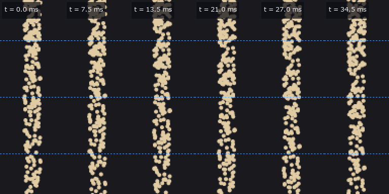
↑ The animation ―― 合成の流れ(3000 個/s、半径 1 mm、幅 8 mm、0.5 mm/px を 2 倍の最近傍、1.5 ms/コマ)。破線 = 流量を読む 3 つの帯。
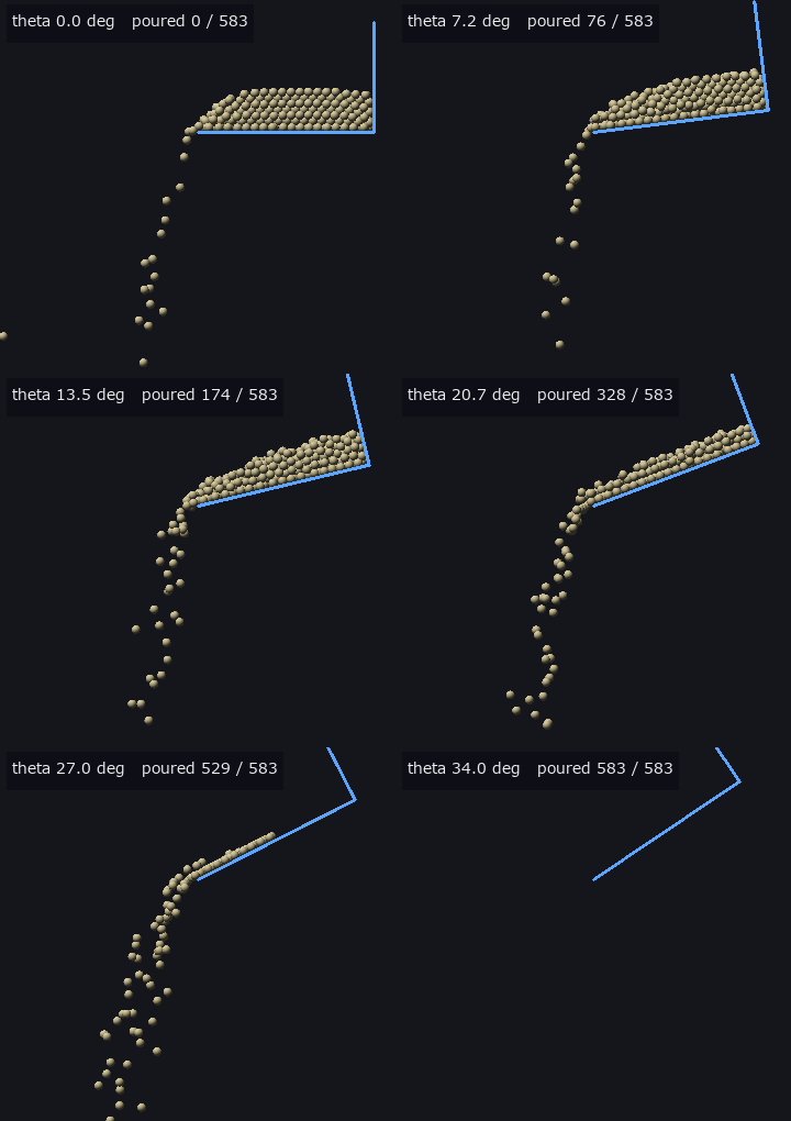
↑ The animation ―― 口の開いた樋(青 = 床と奥壁、床 80 mm、幅 24 mm、滑らかな側壁)を口の縁を軸に 15 度/s で傾ける(剛体球 665 個、0.5 mm/px、陰影つき正射影)。数は傾け始めに器にあった球のうち口を越えた数。
py -3.11 examples/poc_powder_scoop_pour.py
Source: examples/poc_powder_scoop_pour.py
This run produced 12 figures in total - see them all
Ops used (notes): beverloo_rate · difference · heap_volume_cone · pour_scene_mjcf · revolution_volume_side · scoop_count · scoop_image_limit · scoop_scene_mjcf · scoop_synth_side · scoop_volume_read · spheres_render_shaded · spheres_to_silhouette · spoon_bowl_volume · stream_flux_read · stream_synth · text_box · tilt_pour_rate · tilt_wedge_retained · tilted_surface_read · two_view_volume
No.2026.211 —— Measuring Mortar Grinding — D50 of the Size Distribution, Comminution Laws, Spread over Three Independent Runs and AE Band Power, against Published Laser-Diffraction Measurements; a Different D50 Definition Is a One-Bin, 12 % Bias
The physics-simulation × Fullseye series, the third powder exhibit (after granular and scoop). The subject is research in which a robot grinds powder in a mortar and monitors it by acoustic emission (AE). Its published data (Zenodo concept DOI 10.5281/zenodo.18064323, CC BY 4.0) — laser-diffraction size distributions (NaCl / citric acid / monosodium glutamate × three independent runs × seven times from 3 to 25 min, plus before grinding, 60 min and by hand) and six raw AE waveforms — are the outside truth. The data are not in the repo (117 distributions and 6 AE files are extracted and passed via the environment variable FULLSEYE_GRIND_DATA; CI without them runs only the 12 numpy gates). New module grind, 13 ops, no facade. (1) The D50 definition: reading how the instrument CSV pairs bin edges with volume rows, the header’s Dx(50) equals log-diameter linear interpolation of the cumulative at the edges for all 117 files (max difference 3.2e-15). One stage of the published analysis code puts the cumulative at the lower edge and comes out one bin (ratio 1.136) small: −11.80 to −11.98 %. (2) Fitting comminution laws (Reddy’s eqs. (1) and (5)–(7), dE = −C dx/xⁿ: Kick n = 1, Bond 1.5, Rittinger 2) to net grinding time (rms of log D50, 21 points): NaCl Rittinger 0.050, citric acid Bond 0.100, MSG Bond 0.156. Kick is never best. But a Monte Carlo rebuilding the three laws at each material’s times, shrinkage and residual shows how often the true law wins: citric acid 92–100 % (20× shrinkage), MSG 70–92 %, NaCl 58–78 % (2.7×) — NaCl’s “Rittinger is best” cannot be trusted. Extrapolating to before grinding (a measurement not used in the fit): −6 / −18 / −11 % with the best law; with n free it worsens to +34 / +57 % (overfitting). (3) Spread over three independent runs (cv of D50, rms over seven times): NaCl 5.2 %, citric acid 6.5 %, MSG 13.2 %. Repeat measurements of the same powder have cv 0.8–17.1 %, not necessarily smaller than independent runs. At 25 min every pair of materials is more than 12 standard errors apart. (4) The apparent first-order rate of the oversize R(200 µm) (Deniz 2004, after Austin) is 0.17–0.20 /min, slower in the second half (departing from first order). (5) AE band power (0.1–1 MHz) matches the published analysis code run on the same six files with a difference of 0.0, and the band integral of acoustics.stft’s density via Parseval at 0.982–1.052. From 3 to 25 min: NaCl 185 → 31 mV², citric acid 806 → 7.1, MSG 2209 → 184, all in the same direction as D50. (6) At 60 min citric acid is coarser (39.9 µm) than at 25 min (11.4 µm) — agglomeration — and no monotonically fining law can represent it. Figures: synthetic particles with volume vs number basis, law identifiability (synthetic), D50 curves of three materials with three laws, a GIF of the distribution fining, AE spectrograms (start and end on the same colour scale), AE band power vs D50, band power per frame, first-order oversize rate, a table of where the laws break at 60 min, identifiability on the real design. 12 gates (numpy, 0.6 s) plus 10 with data; –full runs 10× the Monte Carlo (25 s with figures). Honestly: energy ∝ net time is an assumption (used only to compare laws). AE has two points per material, so monotonicity and exponents are two-point ratios and no correlation strength can be claimed. The paper’s text, Bond 1952 and Austin’s original were not read. The 60 min and pre-grinding measurements used different instrument settings. D50 from images is gated on synthetic images only.

↑ Measuring Mortar Grinding — D50 of the Size Distribution, Comminution Laws, Spread over Three Independent Runs and AE Band Power, against Published Laser-Diffraction Measurements; a Different D50 Definition Is a One-Bin, 12 % Bias ―― The physics-simulation × Fullseye series, the third powder exhibit (after granular and scoop). The subject is research in which a robot grinds powder in a mortar and monitors it by acoustic emission (AE). Its published data (Zenodo concept DOI 10.5281/zenodo.18064323, CC BY 4.0) — laser-diffraction size distributions (NaCl / citric acid / monosodium glutamate × three independent runs × seven times from 3 to 25 min, plus before grinding, 60 min and by hand) and six raw AE waveforms — are the outside truth. The data are not in the repo (117 distributions and 6 AE files are extracted and passed via the environment variable FULLSEYE_GRIND_DATA; CI without them runs only the 12 numpy gates). New module grind, 13 ops, no facade. (1) The D50 definition: reading how the instrument CSV pairs bin edges with volume rows, the header’s Dx(50) equals log-diameter linear interpolation of the cumulative at the edges for all 117 files (max difference 3.2e-15). One stage of the published analysis code puts the cumulative at the lower edge and comes out one bin (ratio 1.136) small: −11.80 to −11.98 %. (2) Fitting comminution laws (Reddy’s eqs. (1) and (5)–(7), dE = −C dx/xⁿ: Kick n = 1, Bond 1.5, Rittinger 2) to net grinding time (rms of log D50, 21 points): NaCl Rittinger 0.050, citric acid Bond 0.100, MSG Bond 0.156. Kick is never best. But a Monte Carlo rebuilding the three laws at each material’s times, shrinkage and residual shows how often the true law wins: citric acid 92–100 % (20× shrinkage), MSG 70–92 %, NaCl 58–78 % (2.7×) — NaCl’s “Rittinger is best” cannot be trusted. Extrapolating to before grinding (a measurement not used in the fit): −6 / −18 / −11 % with the best law; with n free it worsens to +34 / +57 % (overfitting). (3) Spread over three independent runs (cv of D50, rms over seven times): NaCl 5.2 %, citric acid 6.5 %, MSG 13.2 %. Repeat measurements of the same powder have cv 0.8–17.1 %, not necessarily smaller than independent runs. At 25 min every pair of materials is more than 12 standard errors apart. (4) The apparent first-order rate of the oversize R(200 µm) (Deniz 2004, after Austin) is 0.17–0.20 /min, slower in the second half (departing from first order). (5) AE band power (0.1–1 MHz) matches the published analysis code run on the same six files with a difference of 0.0, and the band integral of acoustics.stft’s density via Parseval at 0.982–1.052. From 3 to 25 min: NaCl 185 → 31 mV², citric acid 806 → 7.1, MSG 2209 → 184, all in the same direction as D50. (6) At 60 min citric acid is coarser (39.9 µm) than at 25 min (11.4 µm) — agglomeration — and no monotonically fining law can represent it. Figures: synthetic particles with volume vs number basis, law identifiability (synthetic), D50 curves of three materials with three laws, a GIF of the distribution fining, AE spectrograms (start and end on the same colour scale), AE band power vs D50, band power per frame, first-order oversize rate, a table of where the laws break at 60 min, identifiability on the real design. 12 gates (numpy, 0.6 s) plus 10 with data; –full runs 10× the Monte Carlo (25 s with figures). Honestly: energy ∝ net time is an assumption (used only to compare laws). AE has two points per material, so monotonicity and exponents are two-point ratios and no correlation strength can be claimed. The paper’s text, Bond 1952 and Austin’s original were not read. The 60 min and pre-grinding measurements used different instrument settings. D50 from images is gated on synthetic images only.

↑ The measurement ―― 同じ画像の同じ粒子でも、体積基準の D50 は個数基準の 1.39 倍。レーザー回折は体積基準。 (figure labels are in Japanese; the numbers are the same)

↑ 縮みが小さいと、雑音 5 % でも 3 則の区別がつかない(200 回ずつ)。

↑ citric acid の D50(独立 3 回)と 3 則の当てはめ。

↑ 各材料 2 点しか取っていない(データ量の上限)ので、傾き α は 2 点の比。

↑ この回の図
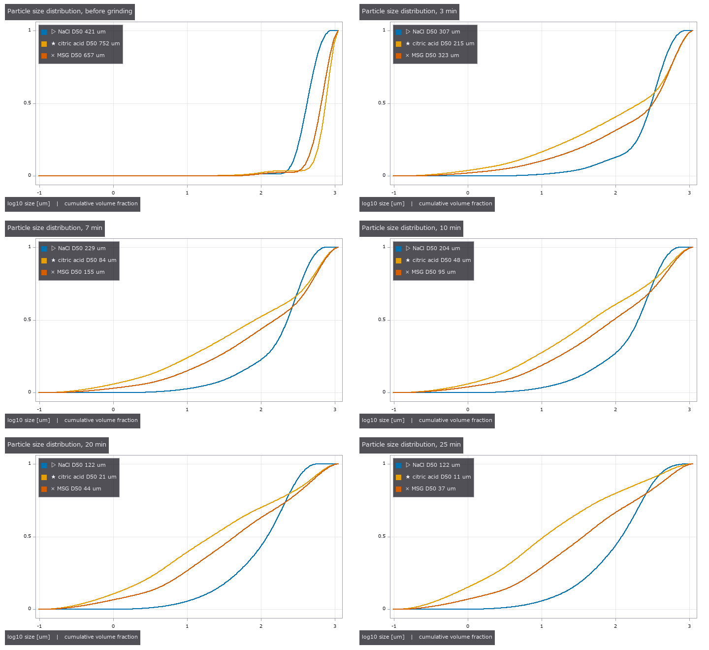
↑ The animation ―― 1st の試行の累積粒度分布が、粉砕前 → 3 → 25 min で左(細かい側)へ動く。
py -3.11 examples/poc_powder_grinding_ae.py
Source: examples/poc_powder_grinding_ae.py
This run produced 13 figures in total - see them all
Ops used (notes): ae_band_power · ae_read_csv · ae_size_correspondence · blob_label · blob_overlay · breakage_first_order_fit · comminution_energy · comminution_law_fit · particle_image_d50 · particle_image_synth · particle_size_dx · particle_size_oversize · particle_size_read · particle_size_synth · replicate_compare
No.2026.215 —— How Long to Grind for a Uniform Dose — Content Uniformity from Particle Size by Closed Form and Monte Carlo, Inverted through Comminution Laws; the Low CV from Photos Was the Same 12 Images at Different Scales
The sequel to grind (measuring mortar grinding). Take one dose from a well-mixed powder and its content varies just because the number of drug particles fluctuates as Poisson. From the compound Poisson process we derive CV² = (πρ/6)·D63³/D (D63 = cube root of the ratio of the 6th to the 3rd number-weighted moment); from a volume-basis size distribution the identity D63³ = E_v[d³] gives it without assuming a shape. Fitting a comminution law to D63 inverts to the grinding time at which the CV reaches a target (6.25 %, equivalent to an acceptance value of 15, or a stage-1 pass probability). Closed form vs Monte Carlo (drawing diameters and summing, no formula): max difference / standard error 1.72 over 8 conditions; identities to 1e-16. ★The pilot run’s “CV from photos is consistently −6 % at four sizes” was an artefact: the four sizes were the same 12 images in pixel units (gate 4). With independent batches the main cause is dropping particles that touch the frame edge (0.956); Miles–Lantuéjoul weights plus a lognormal fit give 1.001 and halve the spread (±0.102 → ±0.060). A powder at CV 6.25 % passes stage 1 only about half the time (chi-square 0.563, 0.501 with the mean-offset term). On published laser-diffraction data (outside the repo, FULLSEYE_GRIND_DATA) a lognormal from D16/D50/D84 overestimates the CV by a median 1,336× (bimodal powders), so it is unusable; reaching CV 6.25 % at 5 mg takes NaCl 24 min, citric acid 28 min and MSG 31 min (the last two extrapolated), and 0.1 mg needs 96–206 min. Honestly: the CV is only the particle-count floor, the acceptance numbers come from secondary sources, and fitting the law to D63 is an assumption. 13 gates (11 on CI without data, 2.3 s); default 1,000 Monte Carlo draws and 30 image batches, –full 8,000 and 200.

↑ How Long to Grind for a Uniform Dose — Content Uniformity from Particle Size by Closed Form and Monte Carlo, Inverted through Comminution Laws; the Low CV from Photos Was the Same 12 Images at Different Scales ―― The sequel to grind (measuring mortar grinding). Take one dose from a well-mixed powder and its content varies just because the number of drug particles fluctuates as Poisson. From the compound Poisson process we derive CV² = (πρ/6)·D63³/D (D63 = cube root of the ratio of the 6th to the 3rd number-weighted moment); from a volume-basis size distribution the identity D63³ = E_v[d³] gives it without assuming a shape. Fitting a comminution law to D63 inverts to the grinding time at which the CV reaches a target (6.25 %, equivalent to an acceptance value of 15, or a stage-1 pass probability). Closed form vs Monte Carlo (drawing diameters and summing, no formula): max difference / standard error 1.72 over 8 conditions; identities to 1e-16. ★The pilot run’s “CV from photos is consistently −6 % at four sizes” was an artefact: the four sizes were the same 12 images in pixel units (gate 4). With independent batches the main cause is dropping particles that touch the frame edge (0.956); Miles–Lantuéjoul weights plus a lognormal fit give 1.001 and halve the spread (±0.102 → ±0.060). A powder at CV 6.25 % passes stage 1 only about half the time (chi-square 0.563, 0.501 with the mean-offset term). On published laser-diffraction data (outside the repo, FULLSEYE_GRIND_DATA) a lognormal from D16/D50/D84 overestimates the CV by a median 1,336× (bimodal powders), so it is unusable; reaching CV 6.25 % at 5 mg takes NaCl 24 min, citric acid 28 min and MSG 31 min (the last two extrapolated), and 0.1 mg needs 96–206 min. Honestly: the CV is only the particle-count floor, the acceptance numbers come from secondary sources, and fitting the law to D63 is an assumption. 13 gates (11 on CI without data, 2.3 s); default 1,000 Monte Carlo draws and 30 image batches, –full 8,000 and 200.

↑ The measurement ―― レーザー回折の粒度分布から形を仮定せずに出した CV(粒の数の揺らぎだけ = 下限)。3 則の必要時間 24〜24 min。目標が測った範囲の近くなので則はほぼ同じ答えを返す。0.1 mg(100〜206 min)のような遠い外挿では則で大きく開く。 (figure labels are in Japanese; the numbers are the same)

↑ レーザー回折の粒度分布から形を仮定せずに出した CV(粒の数の揺らぎだけ = 下限)。

↑ レーザー回折の粒度分布から形を仮定せずに出した CV(粒の数の揺らぎだけ = 下限)。

↑ 同じ粉を挽く時間だけ変えて 5 mg を 10 個取った含量(粒の数の揺らぎだけ、正規近似の 1 回の模擬)。
[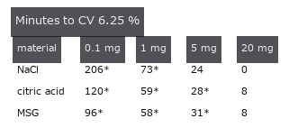](https://raw.githubusercontent.com/furuse-kazufumi/fullseye/master/docs/articles/assets/poc/poc_dose_uniformity_from_grinding/06_grinding_time_by_dose.png)
↑ 最良の則で、CV 6.25 % に要る粉砕時間 [min]。
py -3.11 examples/poc_dose_uniformity_from_grinding.py
Source: examples/poc_dose_uniformity_from_grinding.py
This run produced 7 figures in total - see them all
Ops used (notes): comminution_energy · dose_cv_from_sizes · dose_cv_lognormal · grind_time_for_dose_cv · particle_image_d50 · particle_image_synth · particle_size_read · particle_size_synth
No.2026.216 —— Holding and Cutting with a Knife by Fingertip Visuotactile Sensing Alone — Toughness, Blade Contact Position and How Long a Handle Can Be Held, without a Wrist Force Sensor; the Existing Reader’s Torsion Over-read (+33 % at Half Slip) Fixed by a Numerical Partial-Slip Solution
The chain of cutting (measuring food cutting from images) and pegtactile (contact wrench from two fingertip membranes). Pinch the spine of a kitchen knife between two pads and recover, from the membrane images alone, the push V, the pull H and the moment M_x, then read the blade’s contact position Ly = (M_x + Lz·H)/V, the slice/push ratio ξ̂ = H/V and the toughness R. ★What we found and fixed: pegtactile.pad_tactile_read reads the pad torsion with the no-slip (Reissner–Sagoci) relation, but torsion of a Hertz contact always slips from the edge, so it over-reads M — on partial-slip images ×1.328 at half the full-slip torque and ×2.022 at 0.85 (within 0.4 % of the numerical prediction). Splitting the contact into 64 rings and solving partial slip with the Cerruti-kernel influence matrix (both limits are closed forms: β/β_RS 0.9986 as c → a, the full-slip torque +0.11 % as c → 0) corrects it to within 0.2 %. A MuJoCo cut (4 frames for the default gates, 14 for the figures) → from the pad images alone R̂ 59.86 J/m² (set 60), ξ̂ 0.0701 (tan θ 0.0699), contact position error median 0.01 mm and max 0.48 mm (6.09 mm if the no-slip reading is kept). How long a handle can be held: at a 4 N grip the knife cannot be read once the blade contact is more than 6.0 mm from the grasp (13.2 mm at 8 N, 31.3 mm at 16 N), and outside that range the result carries readable = False. Honestly: the membrane synthesis and the correction use the same numerical solution (whether a real gel behaves like a half-space in partial slip is untested), shear and torsion are superposed, V is the formula written into MuJoCo’s friction loss, and H was made as ξV. 13 gates (3.0 s; without mujoco a closed-form cut stands in); –full runs all 79 frames, 96 rings and 17 positions.
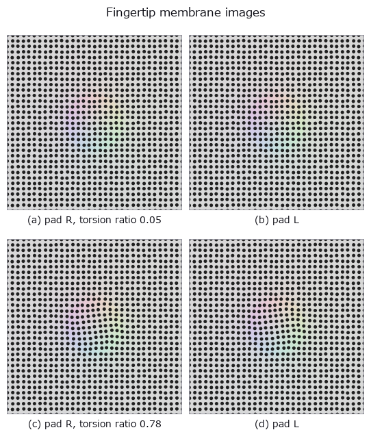
↑ Holding and Cutting with a Knife by Fingertip Visuotactile Sensing Alone — Toughness, Blade Contact Position and How Long a Handle Can Be Held, without a Wrist Force Sensor; the Existing Reader’s Torsion Over-read (+33 % at Half Slip) Fixed by a Numerical Partial-Slip Solution ―― The chain of cutting (measuring food cutting from images) and pegtactile (contact wrench from two fingertip membranes). Pinch the spine of a kitchen knife between two pads and recover, from the membrane images alone, the push V, the pull H and the moment M_x, then read the blade’s contact position Ly = (M_x + Lz·H)/V, the slice/push ratio ξ̂ = H/V and the toughness R. ★What we found and fixed: pegtactile.pad_tactile_read reads the pad torsion with the no-slip (Reissner–Sagoci) relation, but torsion of a Hertz contact always slips from the edge, so it over-reads M — on partial-slip images ×1.328 at half the full-slip torque and ×2.022 at 0.85 (within 0.4 % of the numerical prediction). Splitting the contact into 64 rings and solving partial slip with the Cerruti-kernel influence matrix (both limits are closed forms: β/β_RS 0.9986 as c → a, the full-slip torque +0.11 % as c → 0) corrects it to within 0.2 %. A MuJoCo cut (4 frames for the default gates, 14 for the figures) → from the pad images alone R̂ 59.86 J/m² (set 60), ξ̂ 0.0701 (tan θ 0.0699), contact position error median 0.01 mm and max 0.48 mm (6.09 mm if the no-slip reading is kept). How long a handle can be held: at a 4 N grip the knife cannot be read once the blade contact is more than 6.0 mm from the grasp (13.2 mm at 8 N, 31.3 mm at 16 N), and outside that range the result carries readable = False. Honestly: the membrane synthesis and the correction use the same numerical solution (whether a real gel behaves like a half-space in partial slip is untested), shear and torsion are superposed, V is the formula written into MuJoCo’s friction loss, and H was made as ξV. 13 gates (3.0 s; without mujoco a closed-form cut stands in); –full runs all 79 frames, 96 rings and 17 positions.

↑ The measurement ―― 押し 2 N の切断で、刃の当たり位置が指から離れるほどパッドのねじりが増え、固着円が縮む。把持力 4 N では -3.5〜6.0 mm の外で読めなくなり、-4.5〜7.0 mm の外で全滑り。把持力を 4 倍にすると範囲は約 6.3 倍(全滑りのトルク ∝ P a ∝ P^{4/3})。 (figure labels are in Japanese; the numbers are the same)

↑ 無滑りの関係でねじりを読むと、指から離れるほど当たり位置を遠くに読む(部分滑りでねじれ角が大きい)。

↑ 刃が食材の左端から切れ始め、切っている幅の中点(当たり位置)が右へ動く。

↑ パッドのねじれ(周方向の変位 ÷ 半径)。
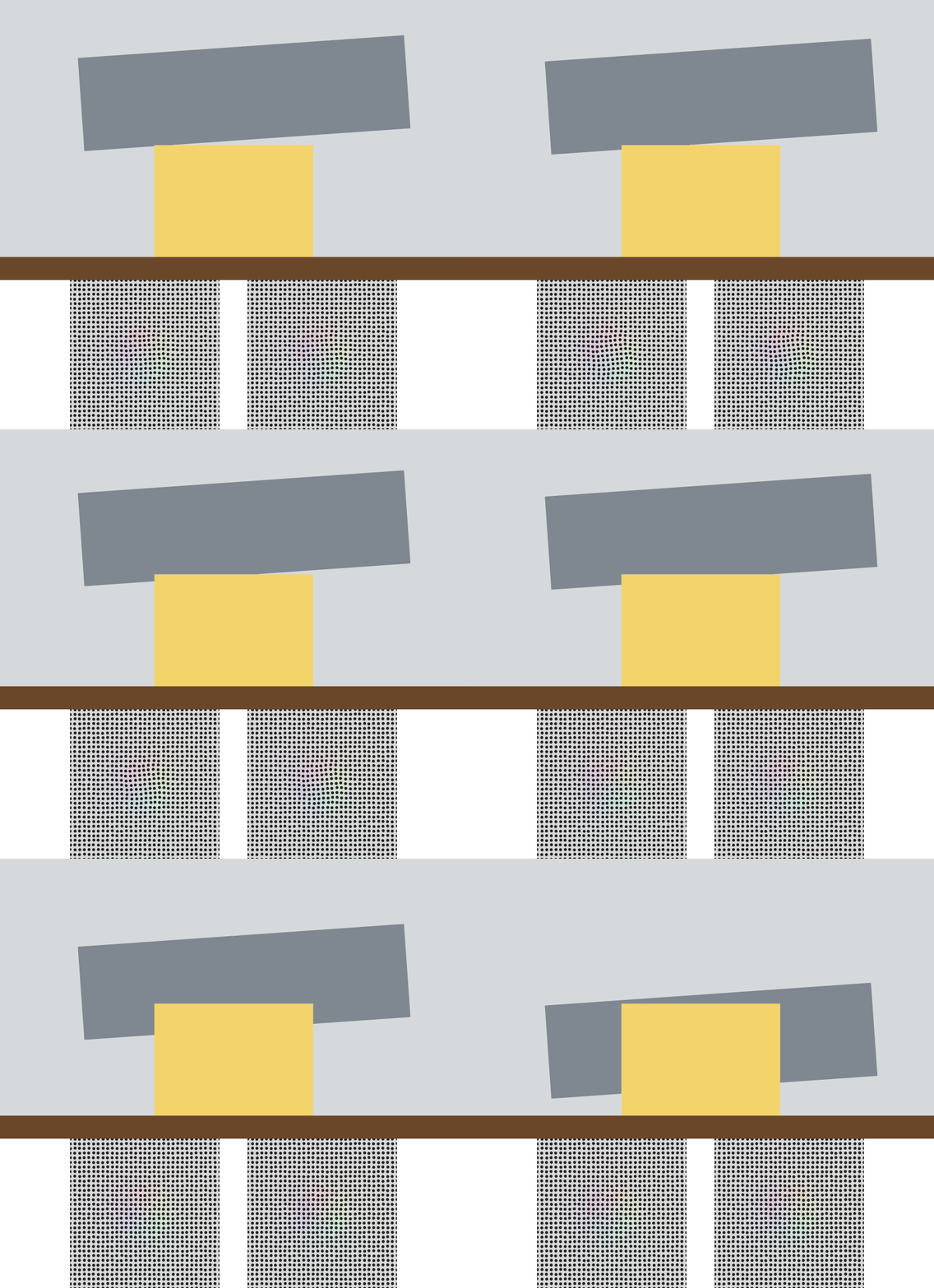
↑ The animation ―― MuJoCo の柔らかい手首で刃を押し下げる(上)。下は包丁の背を挟む 2 枚のパッドの膜の像 —— この像だけで力と当たり位置を読む。
py -3.11 examples/poc_knife_tactile_toughness.py
Source: examples/poc_knife_tactile_toughness.py
This run produced 6 figures in total - see them all
Ops used (notes): combined_modulus · cutting_episode_synth · cutting_scene · food_cut_width · hertz_sphere · knife_load_from_pads · membrane_indent_sphere · membrane_render_markers · membrane_render_rgb · pad_context · pad_marker_displacement · pad_params · pad_tactile_read · peg_wrench_to_pad_loads · rigid_rotation_fit · torsion_partial_slip · toughness_from_pads
No.2026.142 —— How Much of That Number Is Your Measuring - Gauge R&R (gauge repeatability and reproducibility) and Measurement Uncertainty
Separate how much of a number comes from the parts and how much from the act of measuring, then combine the components of one measurement into a reportable uncertainty - scored entirely from outside the picture. The analysis-of-variance decomposition closes algebraically (1e-16); repeatability equals the mean of the per-cell sample variance numpy computes independently; the published worked example is reproduced to 1.5e-06 with contribution percentages 3.4/4.4/7.8/92.2 exactly. Keeping or pooling the interaction moves EV by 7.3 %, so the model actually used is reported; a negative variance component appears in 24 of 40 runs when the true component is zero and is declared, not hidden. Ignoring correlation errs in both directions on the same data (0.0702 -> 0.1945, a 2.8x overestimate, while reactance goes the other way). The effective degrees of freedom are truncated immediately before the t lookup (16.64 -> 16, k = 2.1199). At a stationary point the propagation law returns u = 0 and says so through structure rather than silently; Monte Carlo returns [0, 150]e-6 there. A sum of four rectangular distributions has an exact Irwin-Hall interval of -3.879407, against which the normal approximation is structurally 0.040521 too wide.
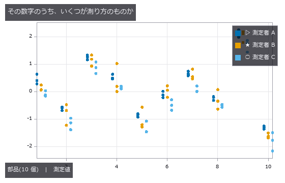
↑ How Much of That Number Is Your Measuring - Gauge R&R (gauge repeatability and reproducibility) and Measurement Uncertainty ―― Separate how much of a number comes from the parts and how much from the act of measuring, then combine the components of one measurement into a reportable uncertainty - scored entirely from outside the picture. The analysis-of-variance decomposition closes algebraically (1e-16); repeatability equals the mean of the per-cell sample variance numpy computes independently; the published worked example is reproduced to 1.5e-06 with contribution percentages 3.4/4.4/7.8/92.2 exactly. Keeping or pooling the interaction moves EV by 7.3 %, so the model actually used is reported; a negative variance component appears in 24 of 40 runs when the true component is zero and is declared, not hidden. Ignoring correlation errs in both directions on the same data (0.0702 -> 0.1945, a 2.8x overestimate, while reactance goes the other way). The effective degrees of freedom are truncated immediately before the t lookup (16.64 -> 16, k = 2.1199). At a stationary point the propagation law returns u = 0 and says so through structure rather than silently; Monte Carlo returns [0, 150]e-6 there. A sum of four rectangular distributions has an exact Irwin-Hall interval of -3.879407, against which the normal approximation is structurally 0.040521 too wide.
Terms: Gauge R&R — A measurement-system analysis in which multiple appraisers repeatedly measure parts to separate equipment repeatability from appraiser reproducibility.
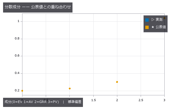
↑ The measurement ―― 測定の行為(GRR)が総変動に占めるのは 7.8 %、部品どうしの差が 92.2 %。どちらも公表値と一致する(最大差 1.5e-06)。 (figure labels are in Japanese; the numbers are the same)
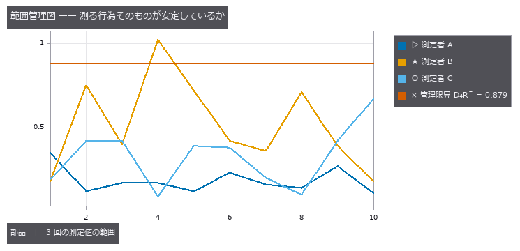
↑ 各升目(部品 × 測定者)で 3 回測った値の幅。
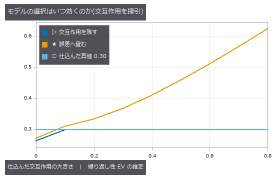
↑ 交互作用が無いところ(左端)では畳むほうが真値 0.30 に近く、あるところでは畳むと交互作用を誤差に混ぜてしまうので上へ外れる。
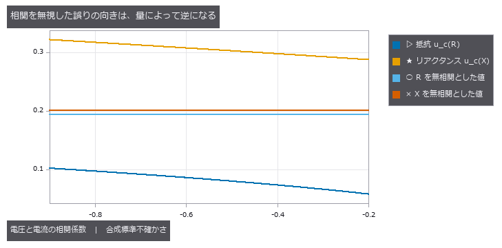
↑ 電圧と電流の相関だけを振った(他の 2 つは実測値で固定)。
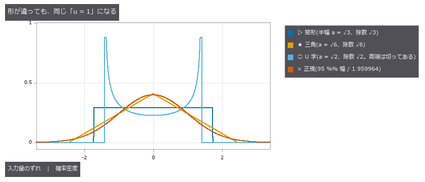
↑ 校正証明書に「±a」とだけ書いてあるとき、それを標準不確かさへ直す除数は形で決まります —— 矩形なら a/√3、三角なら a/√6、両端に寄る U 字(温度の上下動など)なら a/√2、「95 % の幅」と書いてあるなら 1.959964 で割る。
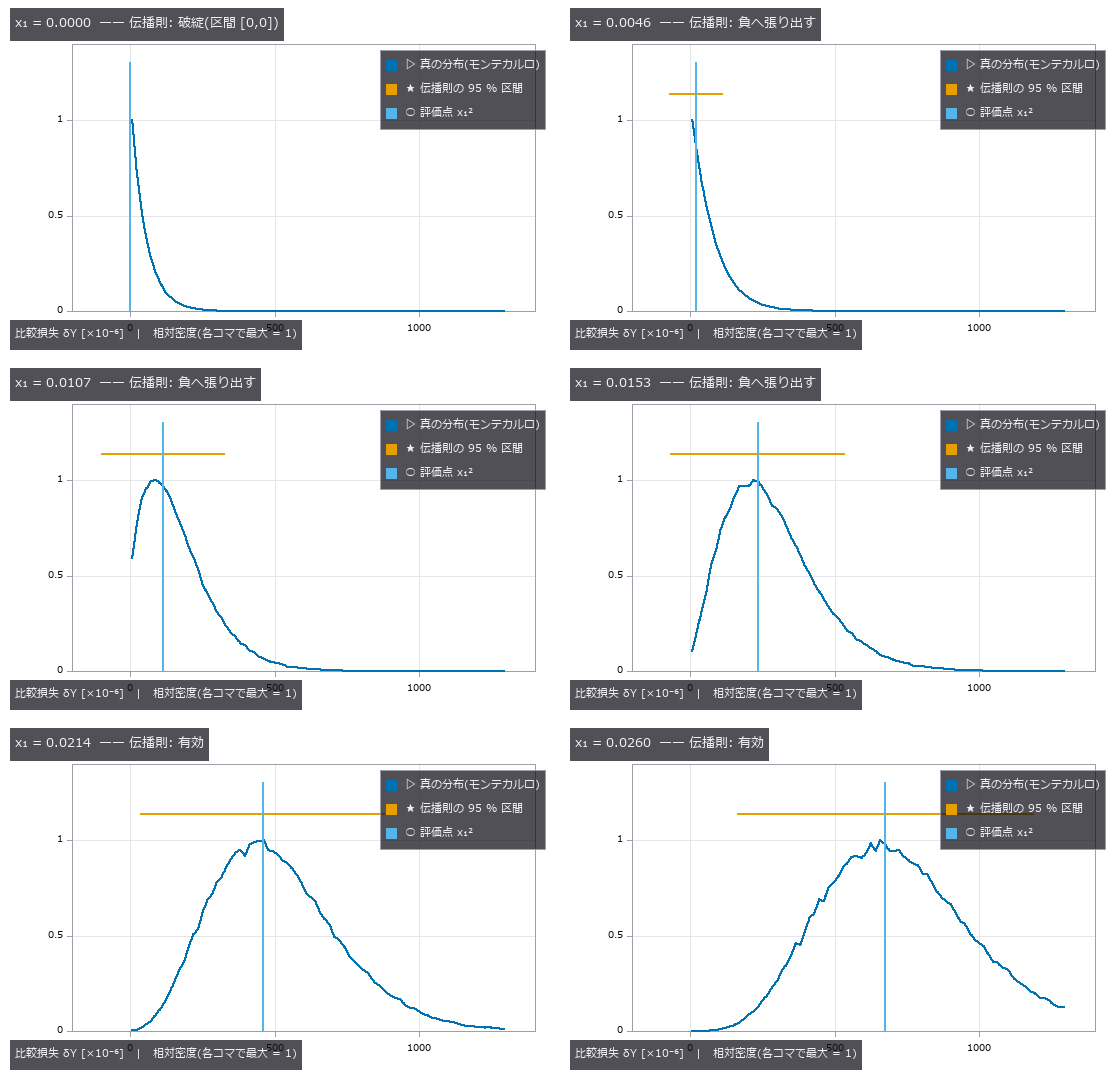
↑ The animation ―― 評価点 x₁ を 0 から 0.026 へ動かしたもの。★左端では真の分布が原点に肩を持つ指数(u²χ²₂)で、伝播則は感度 c = 2x₁ が 0 になるため区間が1 点に潰れる。少し動かすと今度は区間が負の損失へ張り出す(物理的にありえない)。さらに離れると真の分布が正規に近づき、両者はようやく重なる —— 壊れ方は連続ではなく、3 つの段階がある。
py -3.11 examples/poc_measurement_system_analysis.py
Source: examples/poc_measurement_system_analysis.py
This run produced 22 figures in total - see them all
Ops used (notes): axes_frame · axes_transform · grid_lines · gum_expanded · gum_monte_carlo · gum_propagate · gum_standard_uncertainty · gum_validate · legend_box · msa_anova_table · msa_attribute_agreement · msa_bias_linearity · msa_gauge_rr · nice_ticks · plot_series · text_box · ticks
No.2026.219 —— The Resolution Formula Does Not Tell You What You Will Find - Probability of Detection per Lighting (MIL-HDBK-1823A)
V-groove scratches 2-300 µm wide on hairline-finished metal, rendered with the illumination physics, imaged by the same camera and processed by the same chain under three lightings; the truth is the scratch width that was put in. The design formula says the smallest resolvable size is 202 µm, yet with a 70° ring - where the flank mirrors the light into the camera - a90/95 is 8.9 µm, under a dome 27.1 µm, and with a 30° ring 105 of 120 scratches stay below the recording threshold and the a90/95 lies beyond the sizes tested (flagged as extrapolation). Re-rendering 200 scratches at the fitted a90 gives a measured detection rate of 0.910 / 0.845 (band 0.9 +/- 0.064); the hit/miss GLM agrees with the â-vs-a a90 to 0.15 / 0.18 SE; ignoring censoring flattens the slope by up to 4.7 SE; and unflawed sites given random sizes are refused a curve.
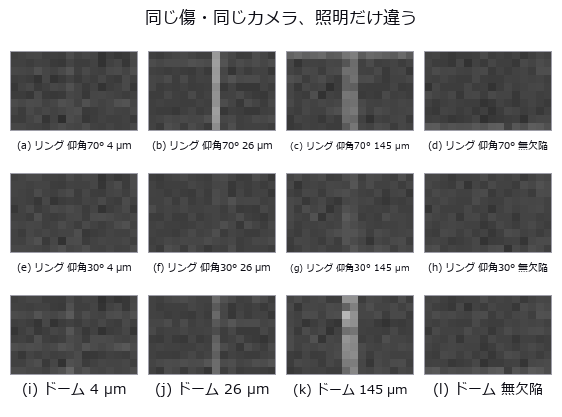
↑ The Resolution Formula Does Not Tell You What You Will Find - Probability of Detection per Lighting (MIL-HDBK-1823A) ―― V-groove scratches 2-300 µm wide on hairline-finished metal, rendered with the illumination physics, imaged by the same camera and processed by the same chain under three lightings; the truth is the scratch width that was put in. The design formula says the smallest resolvable size is 202 µm, yet with a 70° ring - where the flank mirrors the light into the camera - a90/95 is 8.9 µm, under a dome 27.1 µm, and with a 30° ring 105 of 120 scratches stay below the recording threshold and the a90/95 lies beyond the sizes tested (flagged as extrapolation). Re-rendering 200 scratches at the fitted a90 gives a measured detection rate of 0.910 / 0.845 (band 0.9 +/- 0.064); the hit/miss GLM agrees with the â-vs-a a90 to 0.15 / 0.18 SE; ignoring censoring flattens the slope by up to 4.7 SE; and unflawed sites given random sizes are refused a curve.
Terms: POD — A curve giving the probability that a specified inspection procedure detects a flaw as a function of flaw size or another explanatory variable.; a90/95 — The flaw size at which the lower one-sided 95% confidence bound on the POD reaches 90%.
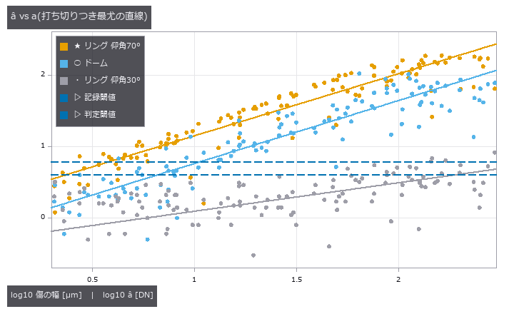
↑ The measurement ―― 記録閾値より下は左打ち切り、応答の天井の 8 割より上は右打ち切りとして尤度に入る(照明ごとに天井が違う)。 (figure labels are in Japanese; the numbers are the same)
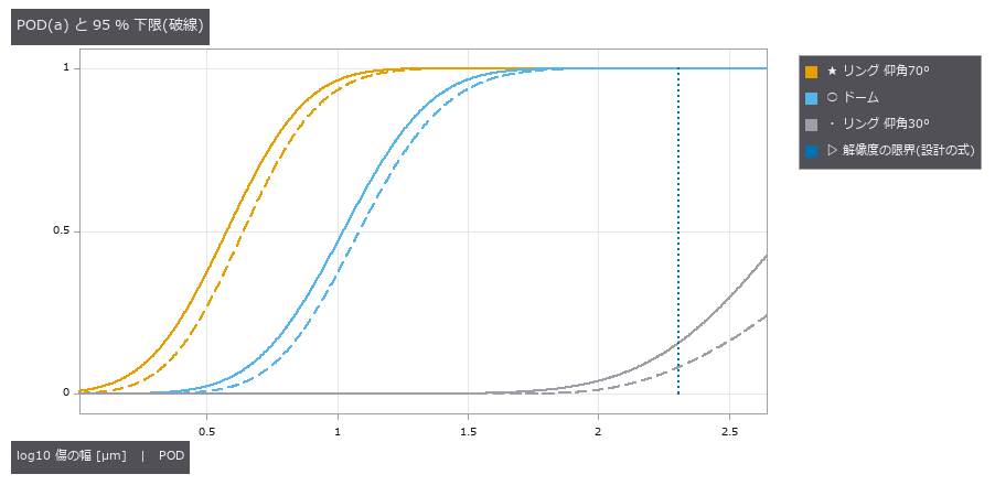
↑ 仰角 70° の a90/95 = 8.9 µm、ドーム 27.1 µm、設計の式の限界 202 µm。
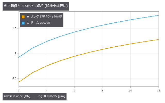
↑ 閾値を上げれば誤検出は減るが、90 % 見つかる大きさは伸びる(1823A 図 G-28)。
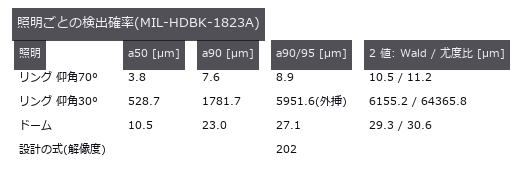
↑ 真値は描画に入れた傷の幅。
py -3.11 examples/poc_pod_lighting.py
Source: examples/poc_pod_lighting.py
This run produced 5 figures in total - see them all
Ops used (notes): light_source · pod_ahat_fit · pod_decision_tradeoff · pod_false_call · pod_from_ahat · pod_hitmiss_fit
No.2026.220 —— Speckle Sets the Error Floor of a Laser Sheet-of-Light - It Does Not Average Away, and the Estimator Ranking Flips
| A sequel to the weld-bead scan: the same laser line, re-rendered by coherent imaging (rough-surface phase, observation pupil, | E | ^2) instead of a smooth band plus additive noise; the truth is the height put into the rendering. The three-point log-parabola that beat the brightest-pixel estimator 8.6-fold under additive noise falls to the brightest pixel’s error under speckle (12.7 vs 13.1 µm) and is twice as bad as the centroid (6.4 µm, 0.93 of Dorsch’s floor C·λ/(2π sin u sin θ) = 6.9 µm) - three samples around the peak follow the brightest grain. Averaging 100 frames of a static part leaves the error at 6.91 -> 6.79 µm; moving the part gives 1/sqrt(N) (0.099). The additive-noise model wrongly promises that averaging helps. Errors over aperture and triangulation angle follow the formula with slopes -0.94 / -0.99 at 0.84-0.90 of its value. Four-times-larger pixels blunt the visible contrast from 1.02 to 0.80 yet move the centroid by 1.6e-13 µm. |

| *↑ Speckle Sets the Error Floor of a Laser Sheet-of-Light - It Does Not Average Away, and the Estimator Ranking Flips ―― A sequel to the weld-bead scan: the same laser line, re-rendered by coherent imaging (rough-surface phase, observation pupil, | E | ^2) instead of a smooth band plus additive noise; the truth is the height put into the rendering. The three-point log-parabola that beat the brightest-pixel estimator 8.6-fold under additive noise falls to the brightest pixel’s error under speckle (12.7 vs 13.1 µm) and is twice as bad as the centroid (6.4 µm, 0.93 of Dorsch’s floor C·λ/(2π sin u sin θ) = 6.9 µm) - three samples around the peak follow the brightest grain. Averaging 100 frames of a static part leaves the error at 6.91 -> 6.79 µm; moving the part gives 1/sqrt(N) (0.099). The additive-noise model wrongly promises that averaging helps. Errors over aperture and triangulation angle follow the formula with slopes -0.94 / -0.99 at 0.84-0.90 of its value. Four-times-larger pixels blunt the visible contrast from 1.02 to 0.80 yet move the centroid by 1.6e-13 µm.* |

↑ The measurement ―― 列ごとの高さの RMS 誤差。加法雑音で最良の 3 点当てはめは、スペックルではいちばん明るい粒を追う。光条全体を平均する重心だけが床に着く。 (figure labels are in Japanese; the numbers are the same)

↑ 部品が止まっていれば 100 枚平均しても誤差はそのまま。

↑ 光条の幅と同じ長さ(48 µm)の束ごとの重心。

↑ θ = 15°〜60°。
py -3.11 examples/poc_laser_line_speckle_floor.py
Source: examples/poc_laser_line_speckle_floor.py
This run produced 5 figures in total - see them all
Ops used (notes): coherent_image · laser_line_coherent · speckle_field · speckle_reduction · speckle_statistics · triangulation_speckle_limit
No.2026.222 —— Fringe Projection Misreads Even a White Groove - Separating the Interreflection, Predicting the Error Before Measuring, and Removing It with Micro Phase Shifting
A white Lambertian part (albedo 0.85, no gloss, no metal) with three 1 mm grooves - a 90 deg inner corner, a 60 deg V-groove and a pocket with rounded corners - measured by fringe projection; the truth is a light-transport matrix (2-D radiosity from Hottel’s crossed-strings form factors) and a direct-only rendering with zero bounces. Shifting stripes parallel to the grooves eight times separates direct and global light (Nayar et al. 2006): the global image glows only inside the concave features, 1.28 times the direct light at the bottom of the inner corner and 5.1 times in the 60 deg groove, within 2.2 % / 6.3 % of the truth; the error falls monotonically from 128 to 8 px stripes and collapses to 54 % at 4 px, narrower than a pixel’s footprint. The fringe phase error is predictable before measuring: the argument of the direct-plus-global phasor from the transport matrix matches the error decoded by wrapped_phase from rendered fringes to 1e-15 rad and never exceeds asin(global/direct). One fringe over a 4 mm field misreads height by 282 / 579 / 183 um RMS; two-level temporal unwrapping (one fringe, then 16 px) picks the wrong order in 329 of 480 pixels (up to 7 orders) and barely helps; micro phase shifting (Gupta & Nayar 2012, periods 16 / 16.2 / 15.8 px, beat 1296 px) brings it to 0.76 / 1.97 / 0.02 um, leaving up to 19 um at the few pixels next to a V vertex. Continuous-wave ToF in a white room corner (4 m, 20 MHz) sees the corner rounded and up to 24 cm too far. Lambertian, extruded (2-D) shapes only; specular interreflection needs Mitsuba and is not modelled.

↑ Fringe Projection Misreads Even a White Groove - Separating the Interreflection, Predicting the Error Before Measuring, and Removing It with Micro Phase Shifting ―― A white Lambertian part (albedo 0.85, no gloss, no metal) with three 1 mm grooves - a 90 deg inner corner, a 60 deg V-groove and a pocket with rounded corners - measured by fringe projection; the truth is a light-transport matrix (2-D radiosity from Hottel’s crossed-strings form factors) and a direct-only rendering with zero bounces. Shifting stripes parallel to the grooves eight times separates direct and global light (Nayar et al. 2006): the global image glows only inside the concave features, 1.28 times the direct light at the bottom of the inner corner and 5.1 times in the 60 deg groove, within 2.2 % / 6.3 % of the truth; the error falls monotonically from 128 to 8 px stripes and collapses to 54 % at 4 px, narrower than a pixel’s footprint. The fringe phase error is predictable before measuring: the argument of the direct-plus-global phasor from the transport matrix matches the error decoded by wrapped_phase from rendered fringes to 1e-15 rad and never exceeds asin(global/direct). One fringe over a 4 mm field misreads height by 282 / 579 / 183 um RMS; two-level temporal unwrapping (one fringe, then 16 px) picks the wrong order in 329 of 480 pixels (up to 7 orders) and barely helps; micro phase shifting (Gupta & Nayar 2012, periods 16 / 16.2 / 15.8 px, beat 1296 px) brings it to 0.76 / 1.97 / 0.02 um, leaving up to 19 um at the few pixels next to a V vertex. Continuous-wave ToF in a white room corner (4 m, 20 MHz) sees the corner rounded and up to 24 cm too far. Lambertian, extruded (2-D) shapes only; specular interreflection needs Mitsuba and is not modelled.
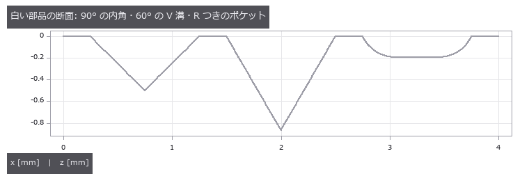
↑ The measurement ―― 反射率 0.85 の Lambert 面。光沢も金属も無い。カメラは真上、プロジェクタは 20° 傾けて縞を溝に平行に投影。 (figure labels are in Japanese; the numbers are the same)

↑ 分離は「大域光が縞の周期より滑らか」という仮定で成り立つ。

↑ 白い Lambert の溝でも数百 µm。

↑ 周期を半分にするたびに誤差は 2〜3 分の 1。

↑ 白い壁(0.8)の 90° の隅を 20 MHz の連続波 ToF で。

↑ The animation ―― 縞をずらしながら撮った 8 枚。縞が当たっていない画素も、溝の中では向かいの面からの光で暗くならない。
py -3.11 examples/poc_interreflection_fringe_error.py
Source: examples/poc_interreflection_fringe_error.py
This run produced 11 figures in total - see them all
Ops used (notes): form_factors_2d · fringe_multipath_phase_error · groove_profile · high_frequency_patterns · micro_phase_decode · predict_fringe_phase_error · render_transport · separate_direct_global · tof_multipath_phase · tof_transport_depth · transport_matrix_radiosity · wrapped_phase
No.2026.150 —— Scoring an Aberration as a Picture: Zernike Polynomials (orthogonal aberration polynomials on a circular pupil) and the Point Spread Function
| A picture of an optical aberration can be scored as a picture: the coefficients can be read back out of it, and what comes back agrees with closed forms. The only operators used are ones already in the box - fit_zernike, which takes a disk image to a dictionary of coefficients, and wavefront_stats, which reports RMS, peak-to-valley and the Strehl ratio. Zernike polynomials form an orthogonal system on the unit disk and are the vocabulary of aberration itself: (2,0) is defocus, (2,+-2) astigmatism, (3,+-1) coma, (4,0) spherical. The twenty-eight modes with n at most six - the closed form (n+1)(n+2)/2 - all equal one exactly at the rim, and the number of radial zeros matches (n- | m | )/2 for every one of them. Orthogonality agrees with the closed form pi/(2(n+1))(1+delta) to 4.86e-06 on the diagonal, with 5.50e-07 off it. The first finding is that the operator’s own disclosure named the wrong cause. Its docstring used to say that at the default sampling up to ten percent leaks between modes, and advised raising the polar resolution. But the leak barely falls with resolution - the ratio per doubling never reaches two. The real cause is the zero background outside the pupil: the outermost ring draws the step into its bilinear interpolation. Extending the polynomial two percent past the rim, which moves the step away from the edge, takes the leak to 0.000041. This finding first corrected the disclosure (2026-10-07) and then the operator itself: since 2026-10-14 its polar grid is area-weighted, with Gauss-Legendre radial nodes that never sit on the rim, and the default worst leak across four modes fell from 0.098 to 0.021. The nodes crowd towards the rim, so discarding the outermost ring only halves what is left (0.0105); removing the step is what removes it. The second finding is that the picture turns while the measurement does not: rotation multiplies each coefficient by a phase, so the paired amplitude is exactly invariant - 1.1e-16 across six angles, and the sum of squares identical to the last bit - and even after drawing the wavefront and reading it back, three rotations spread the amplitude by 2.03e-09. The third is that the rings of the point spread function are set by a Bessel zero: the first dark ring sits at the first zero of J1 divided by pi, 1.219670 in units of lambda over D, and reading it off the picture lands within 3.6e-04 across a threefold range of pupil size. An unaberrated Strehl ratio is exactly one, and the Marechal approximation that wavefront_stats returns differs from the exact diffraction integral by 8.8e-06 at an RMS of 0.02 waves but by 2.0e-02 at 0.18 - a gap that opens by a factor of 2308. The fourth concerns interference fringes: the gradient of spherical aberration vanishes at a radius of one over root two, and the fringes open into a broad band exactly there; measured off the picture the radius comes out at 0.70462 against 0.70711, with the error falling in inverse proportion to the number of fringes. The fifth is that the rotational symmetry of the point spread reveals the azimuthal order, but even orders appear at twice their own frequency. Modes with m of zero are exactly rotationally symmetric; odd orders appear at their own harmonic; even orders vanish there exactly and appear only at twice it - which is why astigmatism looks fourfold rather than twofold. The reason is that an even order makes the wavefront periodic over half a turn, the pupil field centrosymmetric, and the first-order cross term identically zero, so halving the aberration divides the odd harmonics by two and the even ones by four, measured at 2.06 and 3.67. The sixth is that tone mapping is not decoration: rendering the outer rings linearly collapses them to a single level of an eight-bit image, while an inverse hyperbolic sine gives sixty-six - and because that curve is strictly monotone, not one of five thousand sampled pixel pairs changes order. Three predictions were wrong and have been left in, along with two defects in the author’s own measurement. No new operator was added. |
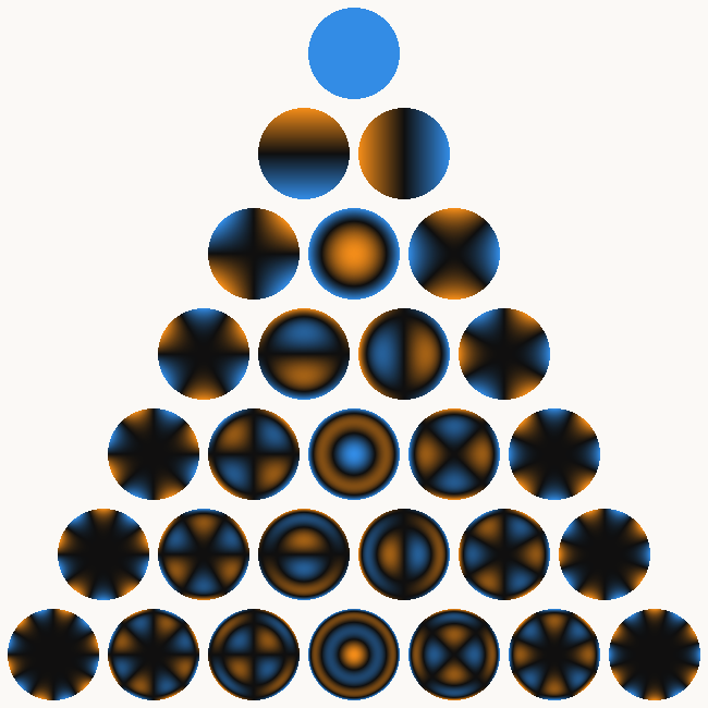
| *↑ Scoring an Aberration as a Picture: Zernike Polynomials (orthogonal aberration polynomials on a circular pupil) and the Point Spread Function ―― A picture of an optical aberration can be scored as a picture: the coefficients can be read back out of it, and what comes back agrees with closed forms. The only operators used are ones already in the box - fit_zernike, which takes a disk image to a dictionary of coefficients, and wavefront_stats, which reports RMS, peak-to-valley and the Strehl ratio. Zernike polynomials form an orthogonal system on the unit disk and are the vocabulary of aberration itself: (2,0) is defocus, (2,+-2) astigmatism, (3,+-1) coma, (4,0) spherical. The twenty-eight modes with n at most six - the closed form (n+1)(n+2)/2 - all equal one exactly at the rim, and the number of radial zeros matches (n- | m | )/2 for every one of them. Orthogonality agrees with the closed form pi/(2(n+1))(1+delta) to 4.86e-06 on the diagonal, with 5.50e-07 off it. The first finding is that the operator’s own disclosure named the wrong cause. Its docstring used to say that at the default sampling up to ten percent leaks between modes, and advised raising the polar resolution. But the leak barely falls with resolution - the ratio per doubling never reaches two. The real cause is the zero background outside the pupil: the outermost ring draws the step into its bilinear interpolation. Extending the polynomial two percent past the rim, which moves the step away from the edge, takes the leak to 0.000041. This finding first corrected the disclosure (2026-10-07) and then the operator itself: since 2026-10-14 its polar grid is area-weighted, with Gauss-Legendre radial nodes that never sit on the rim, and the default worst leak across four modes fell from 0.098 to 0.021. The nodes crowd towards the rim, so discarding the outermost ring only halves what is left (0.0105); removing the step is what removes it. The second finding is that the picture turns while the measurement does not: rotation multiplies each coefficient by a phase, so the paired amplitude is exactly invariant - 1.1e-16 across six angles, and the sum of squares identical to the last bit - and even after drawing the wavefront and reading it back, three rotations spread the amplitude by 2.03e-09. The third is that the rings of the point spread function are set by a Bessel zero: the first dark ring sits at the first zero of J1 divided by pi, 1.219670 in units of lambda over D, and reading it off the picture lands within 3.6e-04 across a threefold range of pupil size. An unaberrated Strehl ratio is exactly one, and the Marechal approximation that wavefront_stats returns differs from the exact diffraction integral by 8.8e-06 at an RMS of 0.02 waves but by 2.0e-02 at 0.18 - a gap that opens by a factor of 2308. The fourth concerns interference fringes: the gradient of spherical aberration vanishes at a radius of one over root two, and the fringes open into a broad band exactly there; measured off the picture the radius comes out at 0.70462 against 0.70711, with the error falling in inverse proportion to the number of fringes. The fifth is that the rotational symmetry of the point spread reveals the azimuthal order, but even orders appear at twice their own frequency. Modes with m of zero are exactly rotationally symmetric; odd orders appear at their own harmonic; even orders vanish there exactly and appear only at twice it - which is why astigmatism looks fourfold rather than twofold. The reason is that an even order makes the wavefront periodic over half a turn, the pupil field centrosymmetric, and the first-order cross term identically zero, so halving the aberration divides the odd harmonics by two and the even ones by four, measured at 2.06 and 3.67. The sixth is that tone mapping is not decoration: rendering the outer rings linearly collapses them to a single level of an eight-bit image, while an inverse hyperbolic sine gives sixty-six - and because that curve is strictly monotone, not one of five thousand sampled pixel pairs changes order. Three predictions were wrong and have been left in, along with two defects in the author’s own measurement. No new operator was added.* |
Terms: Zernike Polynomials — An orthogonal polynomial basis on the unit disk used to decompose pupil wavefront error into terms such as defocus and astigmatism.; PSF — The spatial response of an imaging system to a point object, describing how that point is blurred in the image.; Strehl — An image-quality ratio of the on-axis peak intensity of an aberrated point-spread function to that of the corresponding diffraction-limited system.
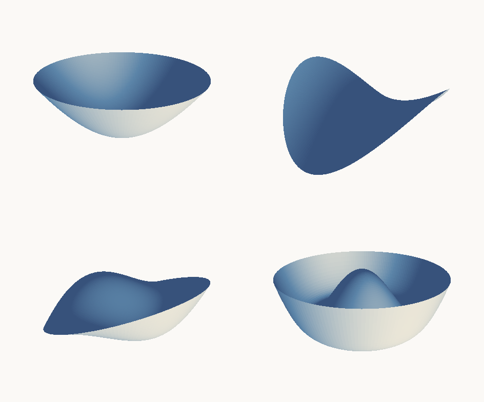
↑ The measurement ―― 波面を立体に起こす(箱の render3d で描画)。左上がデフォーカス(お椀)、右上が非点収差(鞍)、左下がコマ、右下が球面収差。収差の名前は、この形の名前です。立体にしても採点は変わりません —— 係数は絵ではなく多項式に属しているからで、後の図で絵を回しても数が動かないことを見せます。 (figure labels are in Japanese; the numbers are the same)
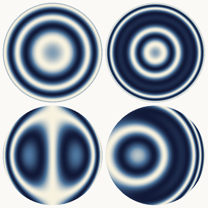
↑ 干渉縞 cos(2πW)。
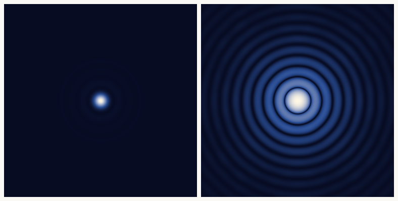
↑ **濃淡の付け方は飾りではありません。
↑ 28 × 28 のグラム行列 ∫Z_n^m Z_n’^m’ ρdρdθ。
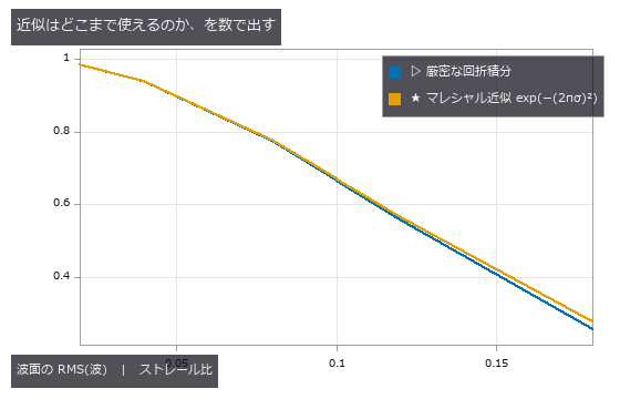
↑ wavefront_stats が返すストレール比はマレシャル近似 exp(−(2πσ)²) です。

↑ The animation ―― スルーフォーカス —— デフォーカスを −0.55 波から +0.55 波まで振って戻します。輪が同心のまま伸縮するのがデフォーカスの特徴で、ピントの前後で絵が対称になります(だから往復させても継ぎ目が見えません)。中央の 1 コマだけが無収差のエアリーで、そこだけストレール比が厳密に 1.000000000000 です。
↑ The animation ―― 絵は回るのに、測った数は動きません。 左が波面(コマ 0.62 + 非点収差 0.35 + 球面収差 0.18)、右がその点像。1 周ぶん回しています。回転は係数を exp(−imθ) 倍するだけなので、対の振幅 √(c₊²+c₋²) は厳密に不変 —— 6 通りの角度で最大 1.1e-16。しかも絵に描いてから fit_zernike で読み返しても、3 通りの回転で振幅の幅は 1.1e-09 しかありません(真値 0.664831)。★球面収差(m = 0)だけは絵そのものが回りません —— m = 0 は回転で変わらないモードだからで、これも絵から読めます。
py -3.11 examples/poc_zernike_aberrations.py
Source: examples/poc_zernike_aberrations.py
This run produced 14 figures in total - see them all
Ops used (notes): fit_zernike · wavefront_stats
No.2026.151 —— Every Speedup Is the Same Arithmetic Regrouped: Scoring Attention with Identities
Every speed and memory trick in the lineage that leads to large language models turns out to be a regrouping of the same arithmetic rather than an approximation, and each identity can be checked to machine precision. The operators are a new family of ten, written in numpy alone - no torch - and the input is a sequence of image patches (a 64 by 64 picture cut into sixty-four eight-by-eight tiles), so attention here is literally the entrance to a vision transformer and the claims hold on the picture side too. The first finding is that tiled attention with an online softmax, the core of FlashAttention, is exact: across seven tile sizes from one row to sixty-four the worst disagreement with the one-pass computation is 1.33e-15. What makes it fast is not a different computation but never forming the T by T matrix at all. A prediction was wrong here: error was expected to accumulate with the number of tiles, and it does, but sixty-four tiles give 1.33e-15 against 1.22e-15 for one - a factor of 1.1. The second is that linear attention is associativity and nothing else: (QK^T)V and Q(K^T V) agree to 1.18e-15, and the causal running-state form to 9.39e-16. The quadratic and linear costs are two bracketings of one product, and the operation counts stand in a ratio of exactly T over d (32 at T of 2048, an integer) – which is why the crossover sits at T equal to d. A second prediction was half right: the measured time ratio stalls at fifteen or sixteen instead of the thirty-two the formula promises, because the quadratic path becomes bandwidth-bound. Time, though, is decided by the machine: the same commit measured 11.6x here and 2.0x on the CI runner, so this PoC gates on the operation-count identity alone and reports the timing without a verdict.
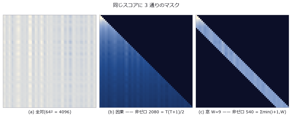
↑ Every Speedup Is the Same Arithmetic Regrouped: Scoring Attention with Identities ―― Every speed and memory trick in the lineage that leads to large language models turns out to be a regrouping of the same arithmetic rather than an approximation, and each identity can be checked to machine precision. The operators are a new family of ten, written in numpy alone - no torch - and the input is a sequence of image patches (a 64 by 64 picture cut into sixty-four eight-by-eight tiles), so attention here is literally the entrance to a vision transformer and the claims hold on the picture side too. The first finding is that tiled attention with an online softmax, the core of FlashAttention, is exact: across seven tile sizes from one row to sixty-four the worst disagreement with the one-pass computation is 1.33e-15. What makes it fast is not a different computation but never forming the T by T matrix at all. A prediction was wrong here: error was expected to accumulate with the number of tiles, and it does, but sixty-four tiles give 1.33e-15 against 1.22e-15 for one - a factor of 1.1. The second is that linear attention is associativity and nothing else: (QK^T)V and Q(K^T V) agree to 1.18e-15, and the causal running-state form to 9.39e-16. The quadratic and linear costs are two bracketings of one product, and the operation counts stand in a ratio of exactly T over d (32 at T of 2048, an integer) – which is why the crossover sits at T equal to d. A second prediction was half right: the measured time ratio stalls at fifteen or sixteen instead of the thirty-two the formula promises, because the quadratic path becomes bandwidth-bound. Time, though, is decided by the machine: the same commit measured 11.6x here and 2.0x on the CI runner, so this PoC gates on the operation-count identity alone and reports the timing without a verdict.
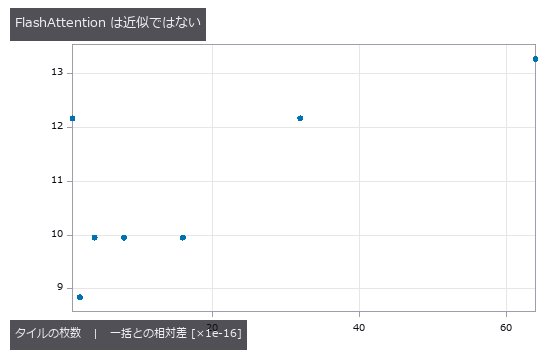
↑ The measurement ―― 縦軸は 1e-16 単位。タイルを 64 枚に割っても相対差は 1.3e-15 —— 近似ではなく、同じ和を別の順で足しているだけ。★外した予言: 誤差はタイル数に比例して積もる → 64 倍のタイル数で 1.1 倍にしかならない。 (figure labels are in Japanese; the numbers are the same)
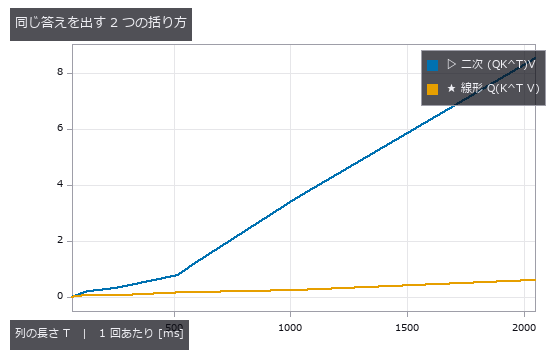
↑ 答えは同じ(相対差 1.2e-15)。
↑ 2 枚目と 3 枚目は差 4.4e-16 —— パッチを並べ替えてから戻すと元に戻る(置換同変)。
↑ 2 本の線は 64 本すべてで重なる(最大差 4.4e-16)。
[](https://raw.githubusercontent.com/furuse-kazufumi/fullseye/master/docs/articles/assets/poc/poc_attention_identities/09_convex_mixing.png)
↑ 行和が 1 なので出力は入力の凸結合で、値域 [0.025, 1.000] を出ない。
py -3.11 examples/poc_attention_identities.py
Source: examples/poc_attention_identities.py
This run produced 10 figures in total - see them all
Ops used (notes): attention_apply · attention_grouped · attention_linear · attention_scores · attention_softmax · attention_tiled · attention_weights · kv_cache_decode · project · rms_norm · rope_rotate
No.2026.218 —— Angles and Shifts No Single Phase Can Pin Down, Fixed by Bundling Phases of Different Periods — the Chinese Remainder Theorem in Images
A phase reports a quantity only modulo its period: a part with four holes cannot tell its orientation apart every 90 degrees, and the phase of a 9 px band cannot tell displacements apart every 9 px. When the periods share no common divisor, the residues fix the value uniquely over their least common multiple (the Chinese remainder theorem) — the same arithmetic Ozaki scheme II uses to rebuild an exact FP64 product from INT8 products. The new family residue (5 ops) is graded in three steps. The theorem: integer CRT (Garner’s mixed radix) matches brute force over all of 0..692, and the real-valued version reproduces it bit for bit on integer input; with one redundant band it names the corrupted band (88.9 % of 3,000 cases) and otherwise answers ‘undecidable’ — never blaming the wrong band. Orientation: a part carrying 3-, 4- and 5-fold rings, each of which folds back every 120 / 90 / 72 degrees on its own (the sawtooth in the figure), is fixed over the full 360 degrees with a maximum error of 0.05 degrees, 0.84 degrees with 40 % of one ring smudged, and the ring with the worst residual pointed at the smudged one 27 of 30 times. Displacement: two regions of the public scikit-image textures moving separately by 20–30 px leave 1.8–2.9 % of the grass pixels far from the boundary off by more than 1 px, against about 50 % for the best pyramid Lucas-Kanade (3–6 levels), 100 % for an ideal single-band phase method, and a single value from global phase correlation. Where it breaks is in the same table: within 1.5 sigma of the boundary (36–85 %), photographs with large flat areas (camera, 23–36 %), and fields that change inside the window (50 % at 6 px amplitude) — a band narrow enough to keep the local frequency stable needs a window too wide to follow the field.
↑ Angles and Shifts No Single Phase Can Pin Down, Fixed by Bundling Phases of Different Periods — the Chinese Remainder Theorem in Images ―― A phase reports a quantity only modulo its period: a part with four holes cannot tell its orientation apart every 90 degrees, and the phase of a 9 px band cannot tell displacements apart every 9 px. When the periods share no common divisor, the residues fix the value uniquely over their least common multiple (the Chinese remainder theorem) — the same arithmetic Ozaki scheme II uses to rebuild an exact FP64 product from INT8 products. The new family residue (5 ops) is graded in three steps. The theorem: integer CRT (Garner’s mixed radix) matches brute force over all of 0..692, and the real-valued version reproduces it bit for bit on integer input; with one redundant band it names the corrupted band (88.9 % of 3,000 cases) and otherwise answers ‘undecidable’ — never blaming the wrong band. Orientation: a part carrying 3-, 4- and 5-fold rings, each of which folds back every 120 / 90 / 72 degrees on its own (the sawtooth in the figure), is fixed over the full 360 degrees with a maximum error of 0.05 degrees, 0.84 degrees with 40 % of one ring smudged, and the ring with the worst residual pointed at the smudged one 27 of 30 times. Displacement: two regions of the public scikit-image textures moving separately by 20–30 px leave 1.8–2.9 % of the grass pixels far from the boundary off by more than 1 px, against about 50 % for the best pyramid Lucas-Kanade (3–6 levels), 100 % for an ideal single-band phase method, and a single value from global phase correlation. Where it breaks is in the same table: within 1.5 sigma of the boundary (36–85 %), photographs with large flat areas (camera, 23–36 %), and fields that change inside the window (50 % at 6 px amplitude) — a band narrow enough to keep the local frequency stable needs a window too wide to follow the field.
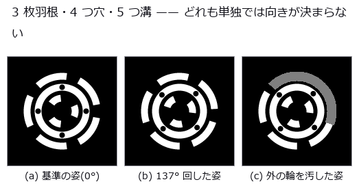
↑ The measurement (figure labels are in Japanese; the numbers are the same)
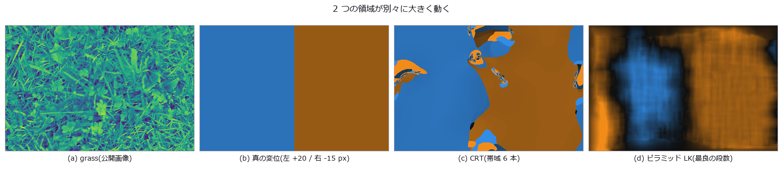
↑ この回の図
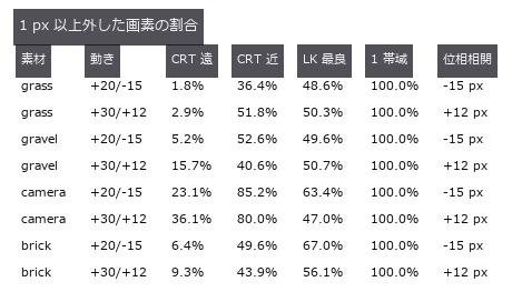
↑ 遠 = 境界から 60 px 以上。
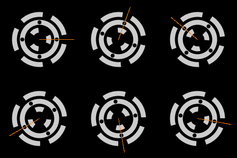
↑ The animation ―― 針 = CRT で決めた向き(1 フレームごとに独立に推定)
py -3.11 examples/poc_residue_crt.py
Source: examples/poc_residue_crt.py
This run produced 5 figures in total - see them all
Ops used (notes): crt_displacement · harmonic_rotation · residue_crt · residue_fault_locate · residue_integer_crt
No.2026.232 —— Moiré (beat fringe between periodic patterns) Alignment — Two Invisible 2 µm Gratings Overlaid Turn a 1 nm Shift into a Readable Fringe Phase
Alignment in lithography and nanoimprint overlays a mask and a wafer to nanometres. Two gratings of slightly different pitch (mask 2.00 µm, wafer 2.04 µm) are each erased by the camera blur (the direct image has a standard deviation of 9e-6), yet overlaid they make 102 µm fringes that magnify the shift fiftyfold. Eight new ops (moirealign, category moire_align of opsoptics): magnification and capture range, the Talbot effect of the proximity gap, the synthetic mark image, the fringe phase by lock-in (least squares at the known frequency) or by Takeda’s FFT method, phase to shift, the differential pair, reading a single, differential or four-quadrant 2-D mark, and the noise lower bound. The magnification depends on which grating moves: measured from the images 50.000 for the wafer and 51.000 for the mask (the often quoted M = p_w/ |
Δp | is the mask-moving case). Eleven 1 nm steps are read with an RMS error of 0.08 nm, and the Monte-Carlo spread matches the phase lower bound (Rife-Boorstyn times the Hann factor 1.5 times 2 for a noisy reference) with a ratio of 1.00. Against the baseline (a resolvable 20 µm bar mark read by cross-correlation and parabolic sub-pixel interpolation) the RMS error is 91 times smaller, but most of that is the parabola’s bias (it reads 17 % short); the random error alone differs only 2.5-fold (0.077 vs 0.19 nm), and the breakdown is printed. With a coarser camera (0.5 to 2 µm pixels) the correlation worsens 2.3-fold while the moiré does not change. Two pairs with opposite pitch differences cancel a 300 nm drift of the whole mark (one pair alone is off by 300/M = 6.2 nm) and a 30 % illumination tilt to within 0.03 nm, and a 2 % camera-scale error moves the reading by 0.007 nm because the conversion depends only on the pitches (the correlation is off by the full 2 %). The reading wraps every pitch (1.01 µm for the differential pair); a coarse correlation fixes the order and reads 0 to 5 µm with 0.14 nm RMS. Across a proximity gap the fringes return at the Talbot length (the lensless self-image distance 2p²/λ) of 14.5 µm and flip sign at half of it, and a flip between reference and measurement makes the reading jump by half a period (1020 nm). Honest limit: the 0.1 nm figures are a white-noise floor; published alignment accuracies of 10 to 30 nm are set by systematic errors such as mark asymmetry, gap and tilt. Nothing learned, nothing calibrated, 32 gates. |
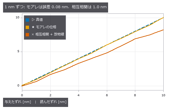
*↑ Moiré (beat fringe between periodic patterns) Alignment — Two Invisible 2 µm Gratings Overlaid Turn a 1 nm Shift into a Readable Fringe Phase ―― Alignment in lithography and nanoimprint overlays a mask and a wafer to nanometres. Two gratings of slightly different pitch (mask 2.00 µm, wafer 2.04 µm) are each erased by the camera blur (the direct image has a standard deviation of 9e-6), yet overlaid they make 102 µm fringes that magnify the shift fiftyfold. Eight new ops (moirealign, category moire_align of opsoptics): magnification and capture range, the Talbot effect of the proximity gap, the synthetic mark image, the fringe phase by lock-in (least squares at the known frequency) or by Takeda’s FFT method, phase to shift, the differential pair, reading a single, differential or four-quadrant 2-D mark, and the noise lower bound. The magnification depends on which grating moves: measured from the images 50.000 for the wafer and 51.000 for the mask (the often quoted M = p_w/ |
Δp | is the mask-moving case). Eleven 1 nm steps are read with an RMS error of 0.08 nm, and the Monte-Carlo spread matches the phase lower bound (Rife-Boorstyn times the Hann factor 1.5 times 2 for a noisy reference) with a ratio of 1.00. Against the baseline (a resolvable 20 µm bar mark read by cross-correlation and parabolic sub-pixel interpolation) the RMS error is 91 times smaller, but most of that is the parabola’s bias (it reads 17 % short); the random error alone differs only 2.5-fold (0.077 vs 0.19 nm), and the breakdown is printed. With a coarser camera (0.5 to 2 µm pixels) the correlation worsens 2.3-fold while the moiré does not change. Two pairs with opposite pitch differences cancel a 300 nm drift of the whole mark (one pair alone is off by 300/M = 6.2 nm) and a 30 % illumination tilt to within 0.03 nm, and a 2 % camera-scale error moves the reading by 0.007 nm because the conversion depends only on the pitches (the correlation is off by the full 2 %). The reading wraps every pitch (1.01 µm for the differential pair); a coarse correlation fixes the order and reads 0 to 5 µm with 0.14 nm RMS. Across a proximity gap the fringes return at the Talbot length (the lensless self-image distance 2p²/λ) of 14.5 µm and flip sign at half of it, and a flip between reference and measurement makes the reading jump by half a period (1020 nm). Honest limit: the 0.1 nm figures are a white-noise floor; published alignment accuracies of 10 to 30 nm are set by systematic errors such as mark asymmetry, gap and tilt. Nothing learned, nothing calibrated, 32 gates.* |
Terms: Moiré — A long-period fringe produced at the difference spatial frequency when two patterns with slightly different pitch or orientation are superposed.
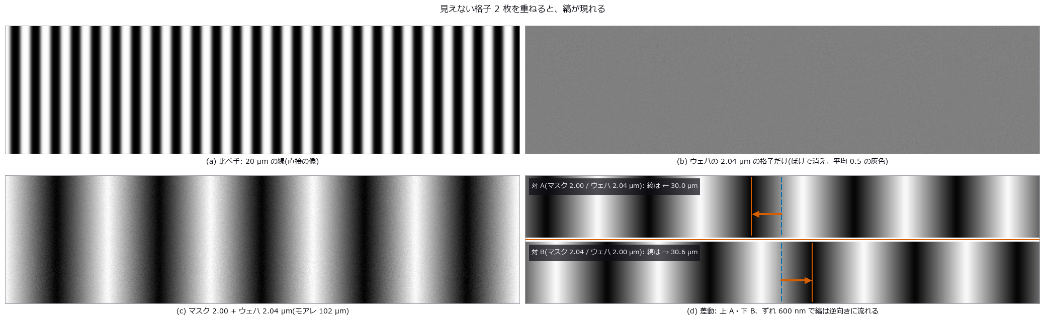
↑ The measurement ―― (a)〜(c) は同じカメラ(画素 0.5 µm、ぼけ σ 1.5 µm)と同じ雑音(σ 0.01)。2 µm の格子はカメラでは消えるが、2 枚の積の差の周波数(1/2.00 − 1/2.04 /µm)だけが残る。(d) は雑音なしの差動のマーク: 橙の線が A と B の境目、青の破線 = ずれ 0 の暗い縞、橙の実線と矢印 = ウェハを 600 nm 動かした後の同じ縞(A は -30.0 µm、B は +30.6 µm)。像全体が流れると両方が同じ向きに動くので、差を取ればずれだけが残る。 (figure labels are in Japanese; the numbers are the same)
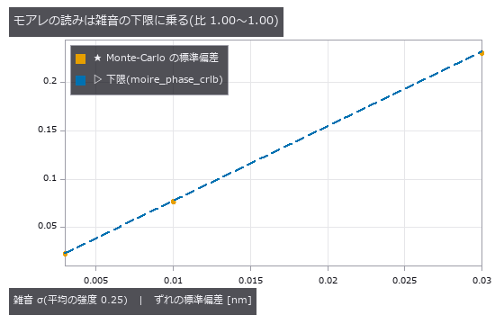
↑ 下限 = Rife & Boorstyn の位相の下限 × Hann の係数 1.5 × 基準像の雑音で 2 倍、を p/(2π) で nm に。
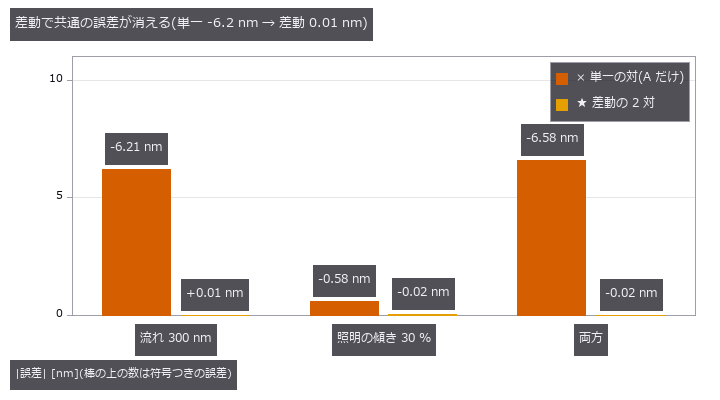
↑ 逆向きのピッチ差の 2 対は、ずれでは逆に、マーク全体の流れでは同じ向きに縞が動く。
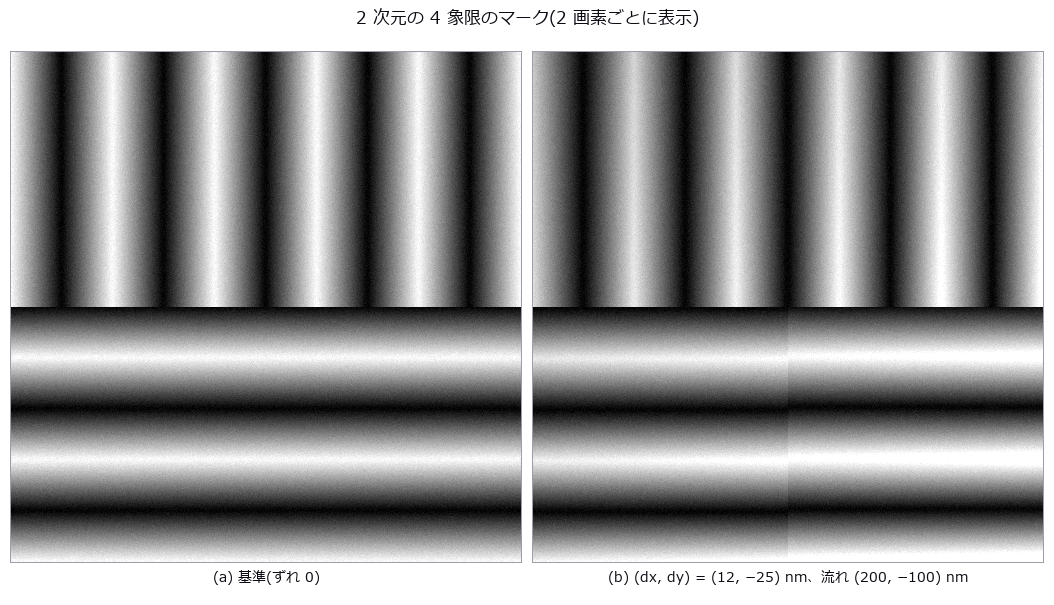
↑ 左上 A_x、右上 B_x、左下 A_y、右下 B_y。
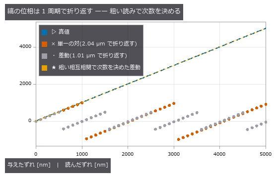
↑ 印刷の版ずれと同じ不定性。
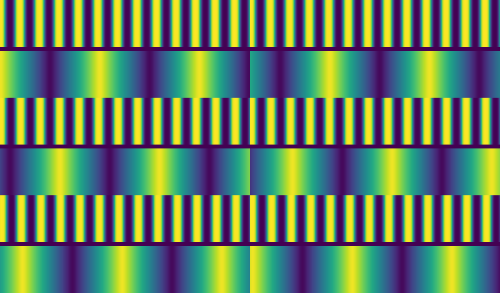
↑ The animation ―― 上: 20 µm の線を直接撮った像、下: モアレ。ずれを 1 コマ 51 nm ずつ、計 2.04 µm(ウェハのピッチ 1 つ)動かす。線は 0.1 画素ずつしか動かず見えないが、縞は 1 コマ 2.55 µm(5 画素)流れ、1 周して元に戻る(= 折り返し)。
py -3.11 examples/poc_moire_alignment.py
Source: examples/poc_moire_alignment.py
This run produced 8 figures in total - see them all
Ops used (notes): arrow · axes_frame · axes_transform · data_to_pixel · grid_lines · legend_box · moire_differential_shift · moire_magnification · moire_mark_read · moire_overlay_image · moire_phase · moire_phase_crlb · moire_phase_to_shift · moire_talbot_gap · nice_ticks · plot_series · text_box · ticks
No.2026.233 —— Telecentric Lenses for Dimensional Metrology — Move Only the Stop of the Same Lens and the Height-Dependent Magnification Disappears
Measured in one image, a stepped part looks larger where it is nearer, so an ordinary lens misreads its dimensions. On the published real images from a telecentric lens, the magnification matched the paper within 0.05 %. In the synthetic chapter, telecentric magnification barely moves with object height.
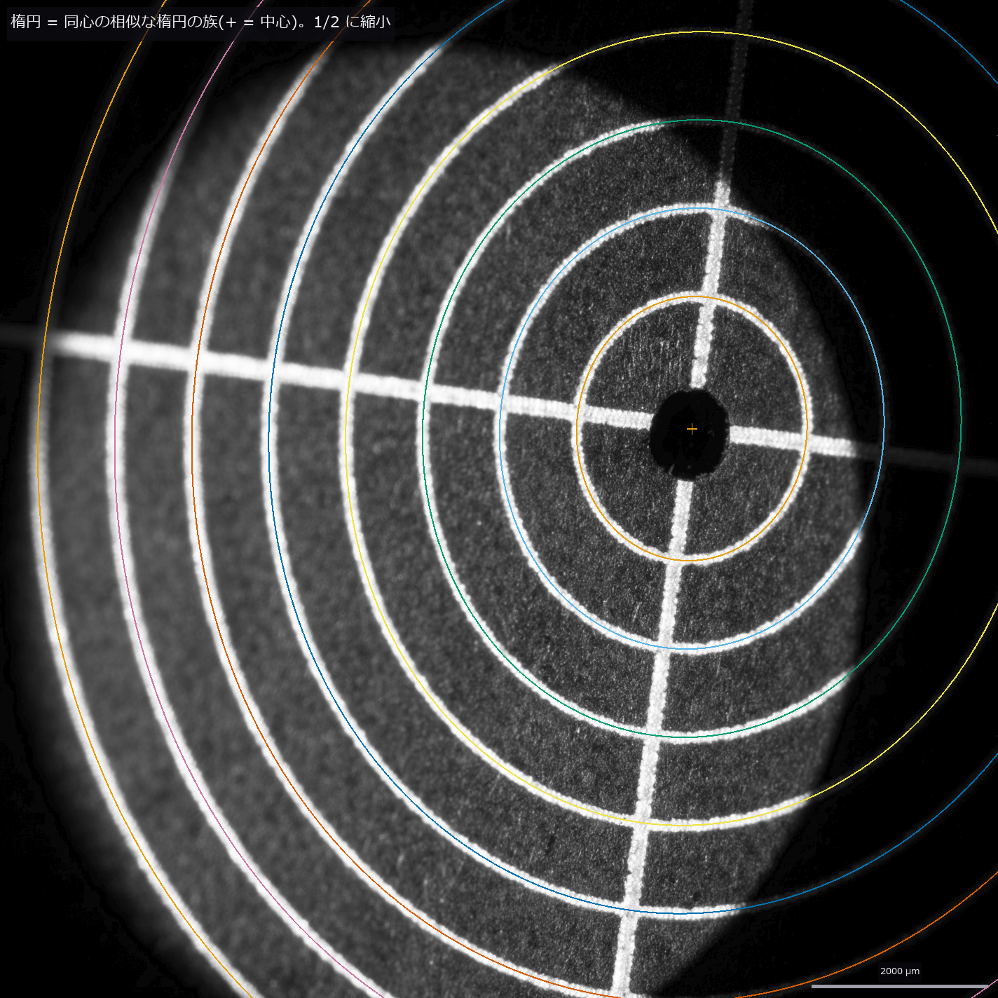
*↑ Telecentric Lenses for Dimensional Metrology — Move Only the Stop of the Same Lens and the Height-Dependent Magnification Disappears ―― The lead chapter measures the paper’s raw telecentric images (Stark et al., Sci. Rep. 15, 28690, 2025, CC BY 4.0) with Fullseye’s metrology ops and checks them against the paper: a family of ellipses sharing one centre and shape, fitted to the eight rings of an alignment plate (1 mm spacing) tilted by 29.5°, gives 252.13 ± 0.04 px/mm along the major axis, +0.05 % from the paper’s K1 = 252.0 px/mm (the paper’s own K1 and K2 spread by ±0.25 %, so the match is not read as finer than that). The telecentric signature: the centres of the concentric rings on the tilted plate do not drift with r² (β = 0.0035 ± 0.0034 px/mm², where a 25 mm entocentric lens would give 1.40 and move the outer centre by 101 px), so the entrance pupil lies beyond 10.5 m. Fitting a free ellipse to each ring instead fails on the outer rings whose arcs are shadowed down to 36–180°. A 3D-printed resin sphere (nominal radius 2.5 mm) is not a usable reference: its outline radius moves 8 % with the threshold. The synthetic chapters that follow sweep the failure conditions. Die bonding and connector-pin inspection measure features at different heights in one image. An ordinary (entocentric) lens magnifies nearer faces more, so the same dimension reads differently above and below a step; a telecentric lens puts the stop at a focal point so the chief rays run parallel to the axis. Seven new ops (telecentric, category telecentric of opsoptics): the same BK7-class singlet (f = 100 mm) with only the stop moved (entocentric, object-side and bi-telecentric), the real chief ray found by aiming at the stop itself so it works with the entrance pupil at infinity (where raytrace.chief_ray stops), magnification versus height, the error across a step, defocus blur, vignetting and a pinhole camera at the entrance pupil for render3d. Moving the object 5 mm closer on a fixed image plane changes the magnification by +6.9 % for a 25 mm machine-vision lens at 75 mm, +1.7 % for the 100 mm entocentric lens and −0.013 % for the telecentric ones; the real rays agree with L/(L − Δz) to 7e-5, and refocusing does not help (m = −f/(s − f) moves by +2.6 %). Rendered through the three lenses, a 5 mm pin top reads 6.9 % too large with the short lens (closed form to 7e-4) and its reading moves 8.6 % over a 6 mm stroke; 2,053 pixels of the bore wall show and only 0.948 of the hole bottom is visible (circle-overlap closed form 0.949), while the bi-telecentric view sees the whole bottom and no wall. The parts are rendered with real material appearance (a brushed aluminium fixture plate, a gold-plated pin, a black moulded package with tinned leads; machining marks and metal colours from complex refractive indices, a clear-coat resin, shadows and ambient occlusion), and under coaxial, dome and low-angle ring lighting a circle metrology model applied to the rendered image reads the pin top within 0.33 % of the closed form, +8.3 to 8.4 % across a 6 mm stroke for the short lens and within ±0.16 % for the bi-telecentric one; at a coarser 47 µm per pixel the low-angle ring reading drifts by 2 % because the dark-field edge is weak. What remains: the singlet’s pupil spherical aberration leaves 0.05° at 8 mm field (growing as h³) and 3 % distortion for the object-side design (0.005 % bi-telecentric); a stop shift moves the entrance pupil to −f²/δ as Newton’s equation says (0.04 % at 0.5 mm field, 11.8 % more at 8 mm); a residual 0.1° shifts a point 9.2 µm across a 5 mm step (closed form 8.7 µm). The front lens sets the field: the 50 % point at 11.6 mm falls 0.8 mm short of the paraxial overlap because pupil aberration shifts and widens the bundle. The blur slope matches |
m | ·NA/√2 within 0.5 %, and NA 0.033 (the smallest that resolves 22 µm) caps the depth of field at 0.68 mm. A second implementation, the open-source optiland, gives the same chief-ray image height to 9e-8 mm (with the same index from a public glass catalogue, so it checks the tracing and aiming code). Nothing learned, nothing calibrated, 29 gates.* |
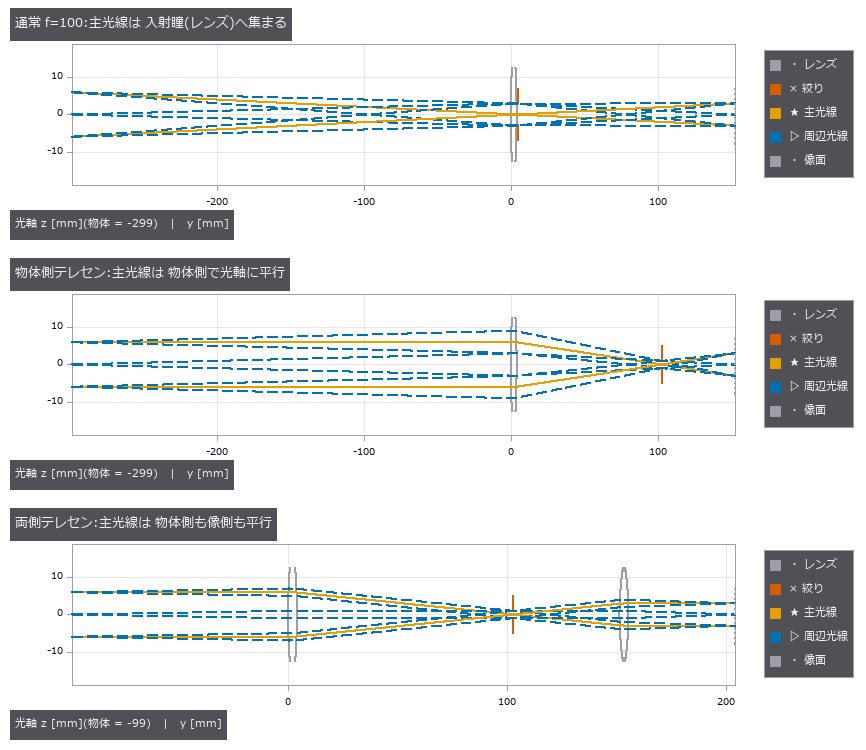
↑ The measurement ―― 同じ BK7 相当の等凸レンズ(f = 100 mm)で、絞り(赤)の位置だけを変えた 3 種。物高 ±6 mm の主光線(実線)は、通常のレンズでは絞りへ向かって傾き、絞りを後側焦点に置くと物体側で光軸に平行になる。 (figure labels are in Japanese; the numbers are the same)
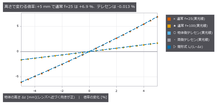
↑ 像面を固定して物体だけを動かした実の主光線の像の高さ。
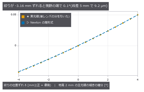
↑ 負 = 主光線が光軸へ寄る(通常のレンズ側)、正 = 遠い物ほど大きく写るハイパーセントリック側。
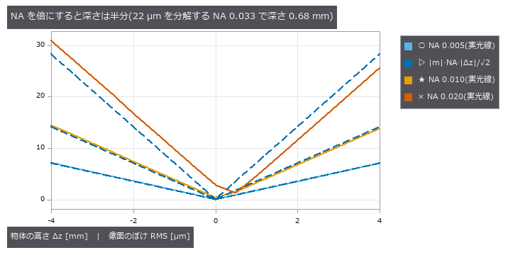
↑ 両側テレセンで NA だけを変えた。
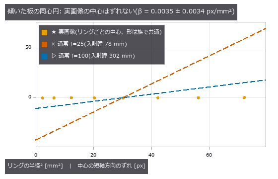
↑ 【実画像】リングごとに形(向き・縦横比・長半径)を族の値に固定して中心だけを解き直し、短軸方向のずれを取った。
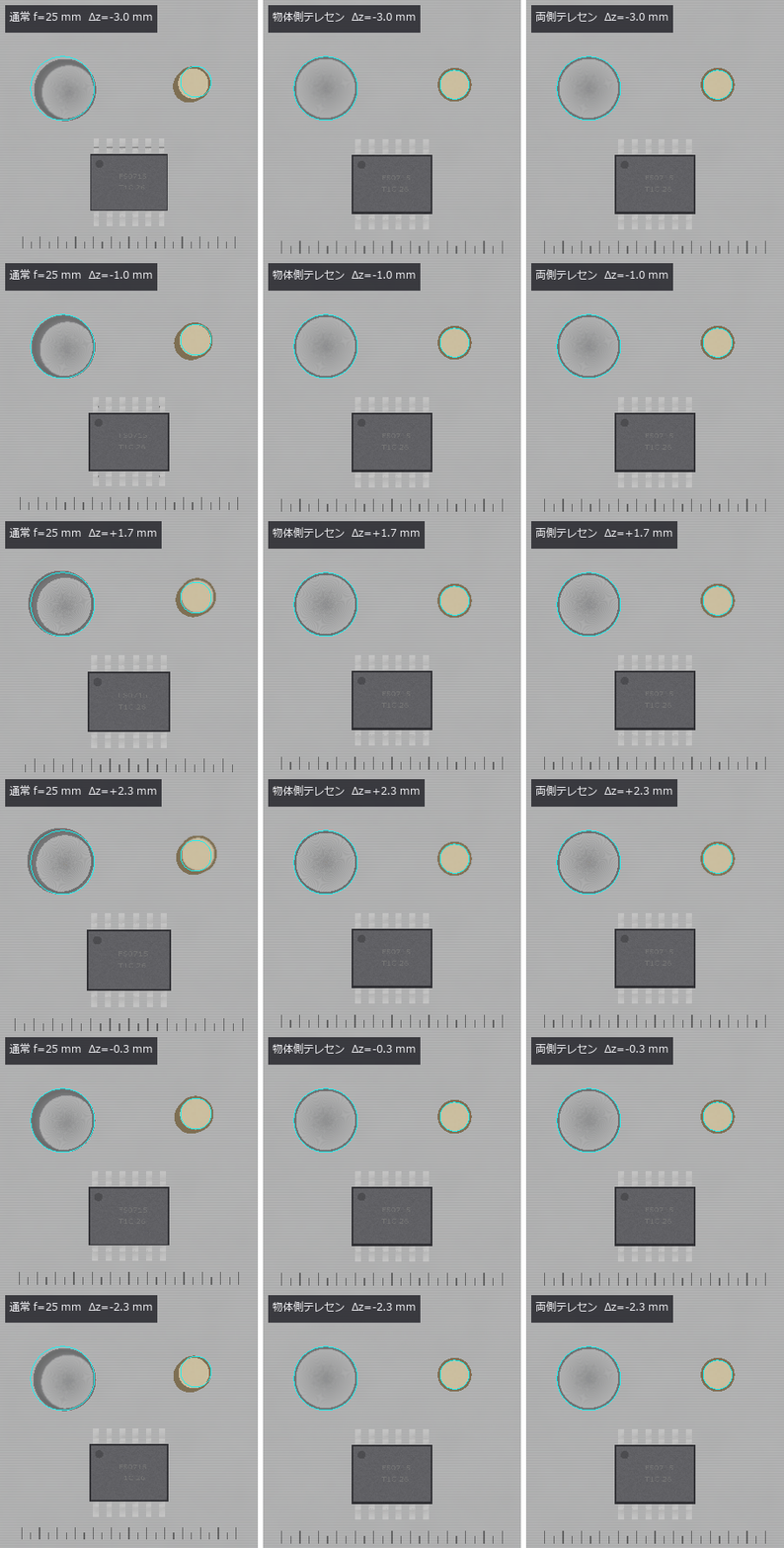
↑ The animation ―― ワークを ±3 mm 上下させる。通常のレンズだけ像が伸び縮みし(水色の線 = 合焦面の輪郭)、穴の底が隠れる。
py -3.11 examples/poc_telecentric_metrology.py
Source: examples/poc_telecentric_metrology.py
This run produced 11 figures in total - see them all
Ops used (notes): add_metrology_object_circle_measure · annotate_scale_bar · apply_metrology_model · blast_normals · cast_shadow · chief_ray · chief_ray_angle · clearcoat_shade · create_metrology_model · defocus_spot_vs_depth · finish_shade · gen_measure_rectangle2 · glass_catalog · lens_equivalent_pinhole · lens_system · magnification_vs_depth · measure_pos · metal_mirror_rgb · micro_normals · paraxial_trace · telecentric_lens · telecentricity_error · text_box · tonemap_reinhard … (+2)
No.2026.242 —— Optical Drawings Straight from the Calculation — Lens Layouts, Vision-Setup Drawings and ISO 10110 Element Drawings as SVG / DXF, Scored by Reading the Written Files Back
In inspection and metrology meetings the lens layout and the setup drawing (working distance, field of view, lighting angles) are the common language, and ordering a lens needs an ISO 10110 element drawing. Fullseye evaluated prescriptions with real rays and produced optical budgets, but drew nothing. Eight new ops (optdraw, category drawing of opsoptics) draw a meridional lens layout (surface sags, edges, stop, image plane, real rays aimed at the stop and coloured by field, EFL / BFL / track / image-height dimensions and a prescription table), a side and top view of a vision setup (field-of-view cone, working distance, depth-of-field band, five light families with elevation angles) and an ISO 10110 three-field element drawing whose tolerances come from the tolerance_analysis dictionary, and write them as SVG (true scale at 100 %) and DXF R12 with layers and line types using only the standard library. The gates score the files read back, not the picture: two textbook Cooke triplets match their published EFL to 7e-6 and 2e-5, drawn surfaces match the closed-form sphere sag to 6e-7 mm, ray kinks lie on the surfaces to 5e-7 mm, chief rays match raytrace.chief_ray to 5e-7 mm and dimension texts match at the printed precision. Telecentric lenses with the entrance pupil at infinity draw too, their chief-ray angles agreeing with telecentric.chief_ray_angle (a separate implementation) to 3e-7 degrees. An open-source DXF library (MIT) read all eleven files with zero audit errors. Inspecting the setup drawing at full size exposed a real bug: the drawn field of view (sensor × WD / f) and the budget magnification f/(WD − f) disagreed by 14 % in the same drawing, because optscene.vision_layout placed the pinhole at the focal length instead of the image distance f·WD/(WD − f); it is fixed, and a gate now counts the pixels of a 12 mm plate in a captured image (124 px against 124.2). Broken drawings turn every gate red. No training, no calibration, 53 gates.
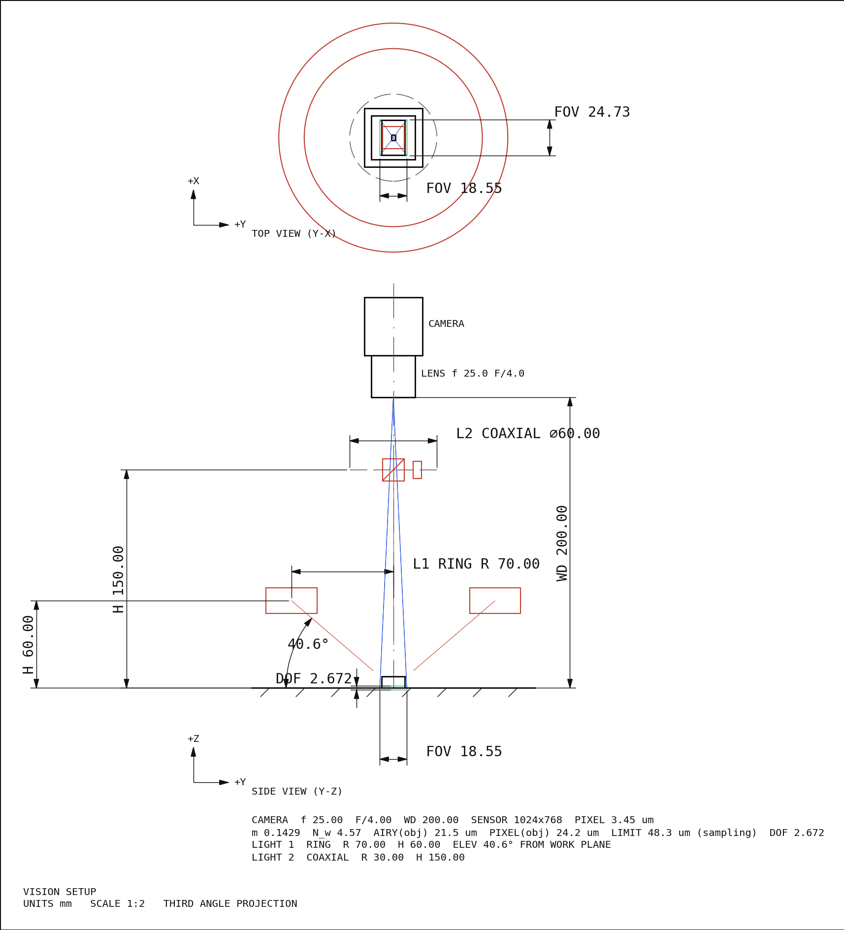
↑ Optical Drawings Straight from the Calculation — Lens Layouts, Vision-Setup Drawings and ISO 10110 Element Drawings as SVG / DXF, Scored by Reading the Written Files Back ―― In inspection and metrology meetings the lens layout and the setup drawing (working distance, field of view, lighting angles) are the common language, and ordering a lens needs an ISO 10110 element drawing. Fullseye evaluated prescriptions with real rays and produced optical budgets, but drew nothing. Eight new ops (optdraw, category drawing of opsoptics) draw a meridional lens layout (surface sags, edges, stop, image plane, real rays aimed at the stop and coloured by field, EFL / BFL / track / image-height dimensions and a prescription table), a side and top view of a vision setup (field-of-view cone, working distance, depth-of-field band, five light families with elevation angles) and an ISO 10110 three-field element drawing whose tolerances come from the tolerance_analysis dictionary, and write them as SVG (true scale at 100 %) and DXF R12 with layers and line types using only the standard library. The gates score the files read back, not the picture: two textbook Cooke triplets match their published EFL to 7e-6 and 2e-5, drawn surfaces match the closed-form sphere sag to 6e-7 mm, ray kinks lie on the surfaces to 5e-7 mm, chief rays match raytrace.chief_ray to 5e-7 mm and dimension texts match at the printed precision. Telecentric lenses with the entrance pupil at infinity draw too, their chief-ray angles agreeing with telecentric.chief_ray_angle (a separate implementation) to 3e-7 degrees. An open-source DXF library (MIT) read all eleven files with zero audit errors. Inspecting the setup drawing at full size exposed a real bug: the drawn field of view (sensor × WD / f) and the budget magnification f/(WD − f) disagreed by 14 % in the same drawing, because optscene.vision_layout placed the pinhole at the focal length instead of the image distance f·WD/(WD − f); it is fixed, and a gate now counts the pixels of a 12 mm plate in a captured image (124 px against 124.2). Broken drawings turn every gate red. No training, no calibration, 53 gates.
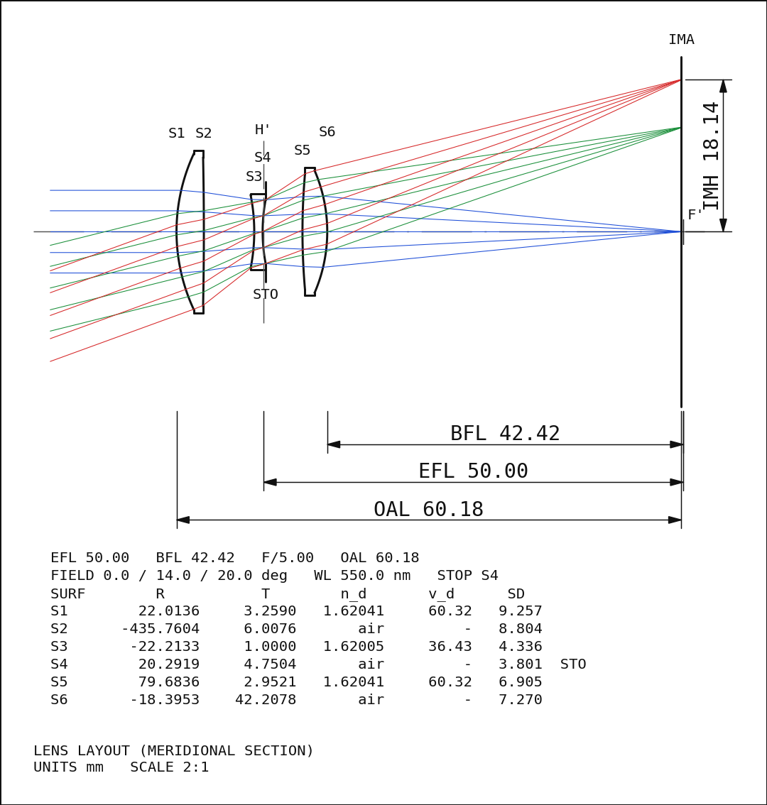
↑ The measurement ―― 教科書の Cooke triplet(f = 50 mm、F/5、半画角 20°)の子午断面。面は処方の sag、光線は絞りを狙って追跡した実光線で、視野 0 / 14 / 20° を青・緑・赤に分けた。寸法線の BFL 42.42・EFL 50.00(H′ → F′)・全長 60.18・像高 18.14 は paraxial_trace の値で、SVG / DXF から読み戻した文字と表示の桁で一致する。縮尺 2:1。 (figure labels are in Japanese; the numbers are the same)
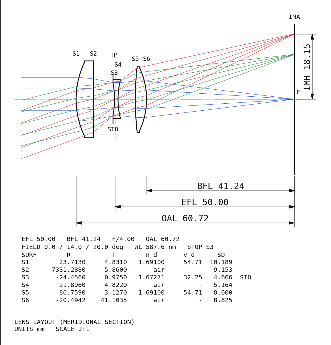
↑ もう 1 本の教科書の Cooke triplet(Geiser の例、f = 50 mm、F/4)。
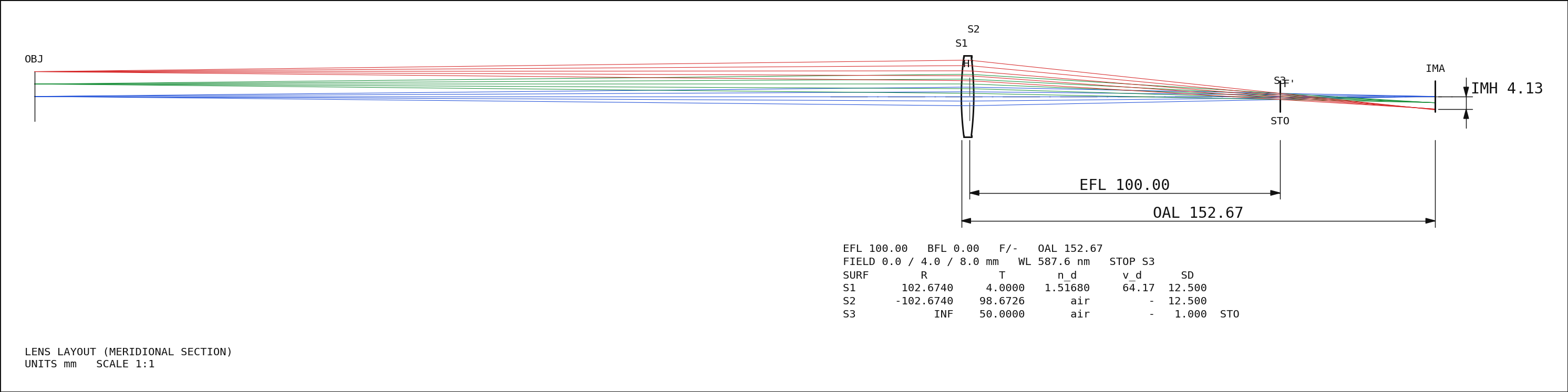
↑ 絞りを後側焦点に置いた物体側テレセン。
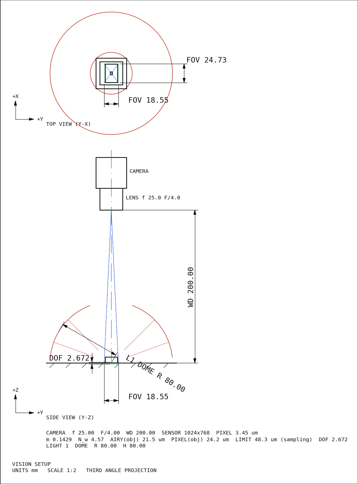
↑ 同じカメラにドーム照明(半径 80 mm、天頂の穴は 20°)。
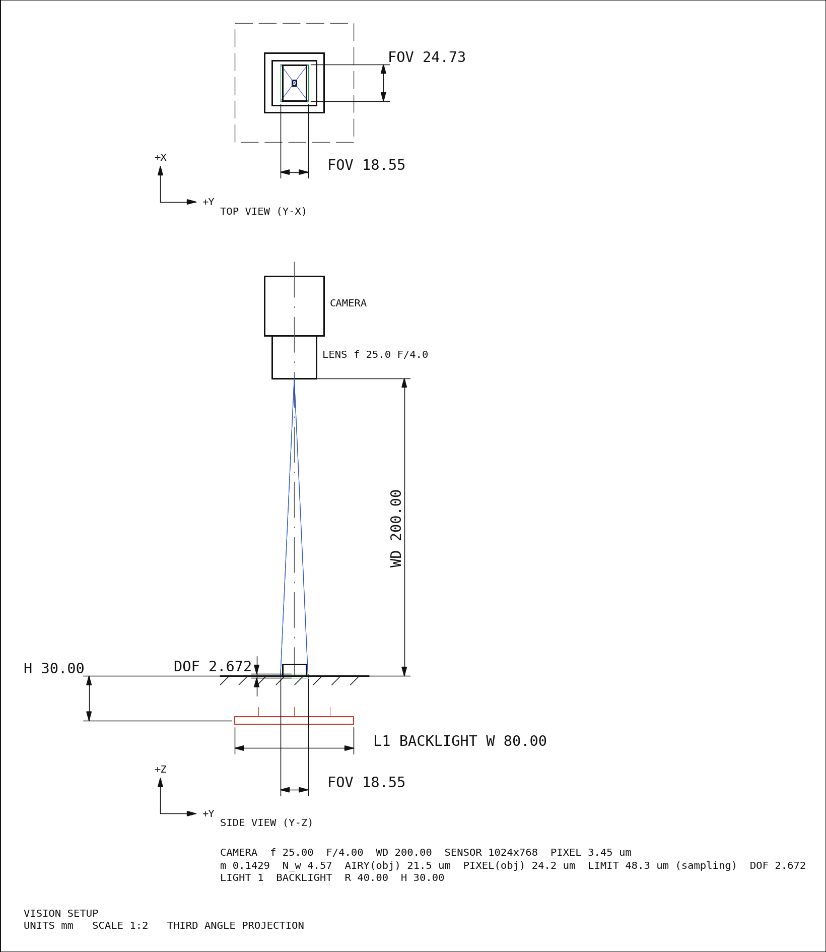
↑ バックライト(部品の下 30 mm、幅 80 mm)。
py -3.11 examples/poc_optics_drawings.py
Source: examples/poc_optics_drawings.py
This run produced 11 figures in total - see them all
Ops used (notes): chief_ray · chief_ray_angle · drawing_dxf · drawing_raster · drawing_svg · dxf_entities · glass · glass_map · layout_capture · lens_element_drawing · lens_section_drawing · lens_spec · lens_system · light_spec · paraxial_trace · scene_box · sensor_spec · svg_entities · telecentric_lens · tolerance_analysis · vision_layout · vision_setup_drawing
No.2026.244 —— Counting Interreflection in a Machined Pocket to Convergence — The Direct-Light Model Fits with Albedo 1.32, the Converged Model Returns the Truth
In a concave part such as a machined pocket, light reflected by one wall lights the floor (interreflection). The inspection renderer render_optscene counts direct light only, and render_studio, which solves interreflection, has no meaningful absolute brightness. Seven new ops (radiosity3d, category radiosity of opsoptics) add render_optscene_gi: the same scene and lights, the direct photometry kept to 1e-16, plus n bounces or the converged sum (Cohen et al. 1988 progressive radiosity, stopped on the residual unshot energy, our choice since the paper gives no number). In a pocket of albedo 0.7, 48 % of the floor’s brightness is interreflection. Calibrating albedo and light intensity with simcal: the direct-only model fits with albedo 1.32 (more light out than in), chi^2/nu 24 and four structured residual components, and is rejected; one bounce gives 0.87 and chi^2/nu 7.9; the converged model returns 0.6996 / 0.9999 (truth 0.70 / 1.00), chi^2/nu 1.01 and white residuals. Seven bounces bring the remainder under the 1.3 % noise (observed ratio 0.51, a GCI-style estimate trusted only in the asymptotic range). Howell’s catalogue values 0.199825 / 0.200044 are reproduced in closed form and numerically, and Table 2 of Bulczak, Lambers and Kolb 2018 (Sensors, CC BY 4.0: one bounce cuts the measured error to 0.20-0.47 of direct-only) is set beside this PoC’s 0.53.
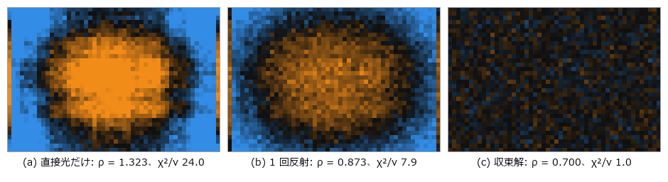
↑ Counting Interreflection in a Machined Pocket to Convergence — The Direct-Light Model Fits with Albedo 1.32, the Converged Model Returns the Truth ―― In a concave part such as a machined pocket, light reflected by one wall lights the floor (interreflection). The inspection renderer render_optscene counts direct light only, and render_studio, which solves interreflection, has no meaningful absolute brightness. Seven new ops (radiosity3d, category radiosity of opsoptics) add render_optscene_gi: the same scene and lights, the direct photometry kept to 1e-16, plus n bounces or the converged sum (Cohen et al. 1988 progressive radiosity, stopped on the residual unshot energy, our choice since the paper gives no number). In a pocket of albedo 0.7, 48 % of the floor’s brightness is interreflection. Calibrating albedo and light intensity with simcal: the direct-only model fits with albedo 1.32 (more light out than in), chi^2/nu 24 and four structured residual components, and is rejected; one bounce gives 0.87 and chi^2/nu 7.9; the converged model returns 0.6996 / 0.9999 (truth 0.70 / 1.00), chi^2/nu 1.01 and white residuals. Seven bounces bring the remainder under the 1.3 % noise (observed ratio 0.51, a GCI-style estimate trusted only in the asymptotic range). Howell’s catalogue values 0.199825 / 0.200044 are reproduced in closed form and numerically, and Table 2 of Bulczak, Lambers and Kolb 2018 (Sensors, CC BY 4.0: one bounce cuts the measured error to 0.20-0.47 of direct-only) is set beside this PoC’s 0.53.
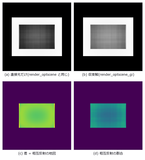
↑ The measurement ―― 同じシーン・同じドーム照明・同じカメラで、直接光だけの検査用描画(左上)と、反射を収束まで数えた描画(右上)。ポケットの底は相互反射で平均 48 % 明るく、角ほど強い(右下は像に占める相互反射の割合)。反射 0 回の render_optscene_gi は render_optscene と 1e-12 以内で一致する。 (figure labels are in Japanese; the numbers are the same)
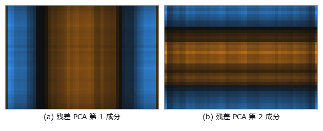
↑ 直接光だけのモデルの残差の主成分(simcal_discrepancy)。
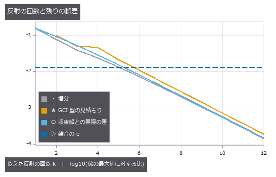
↑ 反射を k 回まで数えた像の誤差。
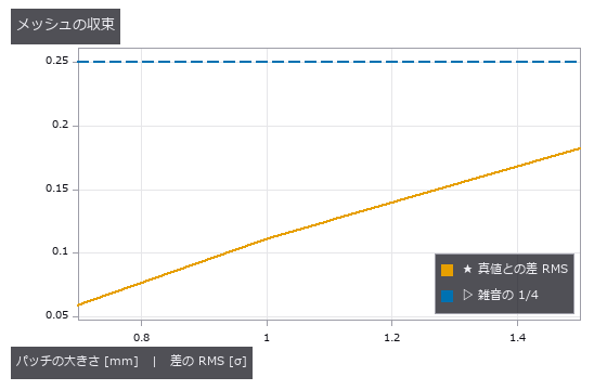
↑ 反射の回数だけでなく、パッチの細かさも収束させる。
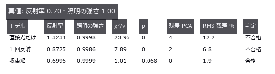
↑ 3 つのモデルを同じ観測(ポケット + 反射率 0.5 の基準の板)に合わせた結果。
py -3.11 examples/poc_pocket_interreflection.py
Source: examples/poc_pocket_interreflection.py
This run produced 7 figures in total - see them all
Ops used (notes): camera_rays · form_factor_matrix · form_factor_parallel_rects · form_factor_perpendicular_rects · form_factor_polygons · intensity · light_source · optical_camera · radiosity_patches · radiosity_progressive_3d · render_optscene · render_optscene_gi · scene_box · scene_difference · scene_material · scene_plane · simcal_discrepancy · simcal_fit · simcal_model · simcal_observe · simcal_simulate · simcal_validate · trace_rays
No.2026.248 —— Non-Coaxial Optics — a Coaxial-Illumination Beamsplitter Paints a False Defect on a Mirror-Like Part, Removed by a Coating or a Wedge; Fold Mirrors Shrink the Machine
Inspection optics rarely keep one straight axis: coaxial epi-illumination looks through a 45° beamsplitter, fold mirrors shrink the machine, and a tilted sensor brings a tilted part into focus. raytrace traced coaxial systems only and could not compute the ghost a beamsplitter’s back face makes. Thirteen new ops (raytrace3d, category noncoaxial) and optdraw.noncoaxial_drawing give every surface a 3-D pose (coordinate breaks decenter, then rotate x → y → z; undo reverses them) and trace with raytrace’s own surface equations: eight coaxial prescriptions match raytrace.trace_rays exactly (within 1e-12). A 45° fold reproduces the Householder mirror image of the unfolded image to 3e-14 mm, one reflection reverses the image and two restore it, and folding the camera arm of a coaxial inspection lens with two mirrors cuts the height from 393 to 249 mm with an unchanged image. Tilted-plate shift (Smith) matches real rays to 1e-12 mm and astigmatism (Coddington; the tangential image lies farther) to 1e-6 mm, and the Scheimpflug image tilt tan θ’ = m tan θ to 2e-4 degrees. The two-reflection ghost between the beamsplitter’s back and front faces carries 2.6 % of the image (Fresnel at 28° to 1e-6) and lays a shifted copy of a dent on a mirror-like part (m × 2t tan θ’ cos θ = 2.6 mm); a simple detector reports it as a false dent 0.010 mm from the predicted spot. A quarter-wave MgF2 layer only reaches 2.1 % at 45°; a two-layer coating tuned for the angle (0.38 %) drops the ghost to 0.19 % and the false dent disappears, and a 1° wedge throws the ghost 9.5 mm off the sensor. As a second implementation the open-source tracer optiland (MIT), built with the same absolute surface poses, agrees on every surface intersection of six systems to 1e-13 mm (CI checks recorded values to 1e-7 mm). Broken frames, fold orders and ghost paths turn the gates red. No training, no calibration, 19 gates.
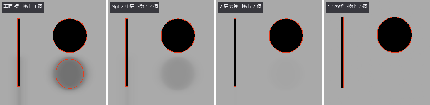
↑ Non-Coaxial Optics — a Coaxial-Illumination Beamsplitter Paints a False Defect on a Mirror-Like Part, Removed by a Coating or a Wedge; Fold Mirrors Shrink the Machine ―― Inspection optics rarely keep one straight axis: coaxial epi-illumination looks through a 45° beamsplitter, fold mirrors shrink the machine, and a tilted sensor brings a tilted part into focus. raytrace traced coaxial systems only and could not compute the ghost a beamsplitter’s back face makes. Thirteen new ops (raytrace3d, category noncoaxial) and optdraw.noncoaxial_drawing give every surface a 3-D pose (coordinate breaks decenter, then rotate x → y → z; undo reverses them) and trace with raytrace’s own surface equations: eight coaxial prescriptions match raytrace.trace_rays exactly (within 1e-12). A 45° fold reproduces the Householder mirror image of the unfolded image to 3e-14 mm, one reflection reverses the image and two restore it, and folding the camera arm of a coaxial inspection lens with two mirrors cuts the height from 393 to 249 mm with an unchanged image. Tilted-plate shift (Smith) matches real rays to 1e-12 mm and astigmatism (Coddington; the tangential image lies farther) to 1e-6 mm, and the Scheimpflug image tilt tan θ’ = m tan θ to 2e-4 degrees. The two-reflection ghost between the beamsplitter’s back and front faces carries 2.6 % of the image (Fresnel at 28° to 1e-6) and lays a shifted copy of a dent on a mirror-like part (m × 2t tan θ’ cos θ = 2.6 mm); a simple detector reports it as a false dent 0.010 mm from the predicted spot. A quarter-wave MgF2 layer only reaches 2.1 % at 45°; a two-layer coating tuned for the angle (0.38 %) drops the ghost to 0.19 % and the false dent disappears, and a 1° wedge throws the ghost 9.5 mm off the sensor. As a second implementation the open-source tracer optiland (MIT), built with the same absolute surface poses, agrees on every surface intersection of six systems to 1e-13 mm (CI checks recorded values to 1e-7 mm). Broken frames, fold orders and ghost paths turn the gates red. No training, no calibration, 19 gates.
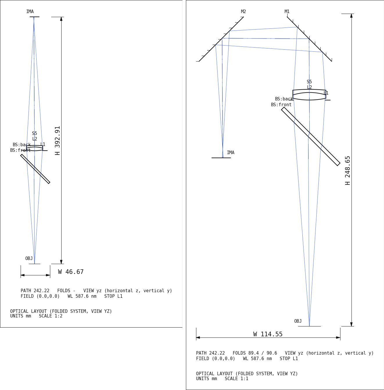
↑ The measurement ―― 同軸落射の検査レンズ(物体 → 45° の半透鏡 → 2 枚玉 → カメラ)の設置図。左はまっすぐ、右はカメラ側を 2 枚の 45° の鏡で折った版で、装置の高さが 393 → 249 mm に縮む。像の RMS は変わらない(門)。図は noncoaxial_drawing が大域の座標で描いた実寸の断面で、光線は絞り(L1)を狙った実光線。 (figure labels are in Japanese; the numbers are the same)
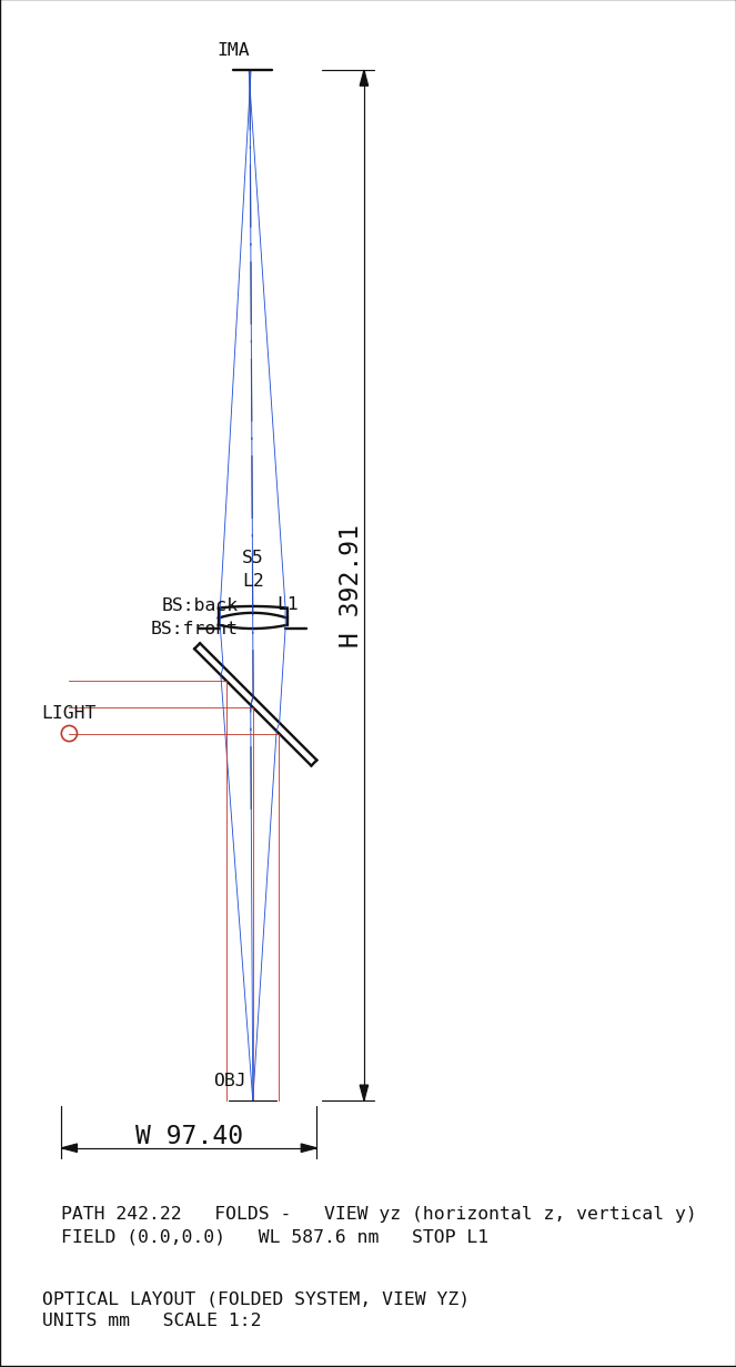
↑ 同軸落射の光学系: 横から来る照明(赤)を半透鏡が真下の部品へ曲げ、部品で鏡面反射した光が半透鏡を透過して2 枚玉に入る(青)。

↑ 集光する光束(f/25)に 5 mm の平板を傾けて入れたときの、主光線の横ずれと、接線像と球欠像の距離(非点隔差)。
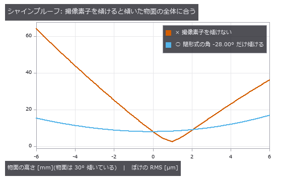
↑ 2 枚玉(f ≈ 100 mm)で 200 mm 先の 30° に傾いた面を撮る。
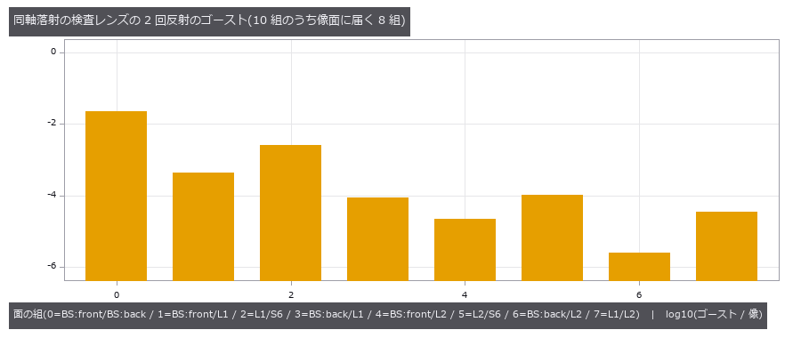
↑ 全ての 2 面の組(N(N−1)/2 = 10)のうち、像面に光が届く組の、像に対するエネルギー比(届く割合を掛けた値)。
py -3.11 examples/poc_noncoaxial_optics.py
Source: examples/poc_noncoaxial_optics.py
This run produced 6 figures in total - see them all
Ops used (notes): beamsplitter_branches · drawing_raster · ghost_analysis · ghost_image · ghost_path · image_orientation · lens_system · noncoaxial_drawing · noncoaxial_example · noncoaxial_layout · noncoaxial_spot · noncoaxial_system · noncoaxial_trace · opd_samples · paraxial_trace · ray_bundle · scheimpflug_tilt · surface_reflectance · text_box · tilted_plate_shift · trace_rays
No.2026.253 —— Calibrating an Imaging Model on a Real Telecentric Image — the Scale Matches the Paper, the Entrance Pupil Is Only ‘Farther than 1 m’
An imaging model with plate tilt, orientation, scale, radial distortion k1 and the inverse entrance-pupil distance 1/L (telecentricity) is calibrated with simcal on the ring centrelines of a real 29.5-degree tilted alignment plate (Stark et al., Sci. Rep. 2025, CC BY 4.0). With a noise level independent of the model (local-quadratic pure error, 1.12 px) the absolute chi-square gate fails (p = 7e-9) and the numbers are withdrawn: the 1.35 px residual carries smooth ring-by-ring discrepancy. Adding it as white variance passes all six gates, and only after checking that a ring jackknife agrees with the Laplace uncertainty are numbers reported: 252.14 ± 0.18 px/mm (paper K1 = 252.0) and 1/L = 0.50 ± 0.18 per metre, i.e. the entrance pupil is farther than 1.16 m (2 sigma), which rules out the ordinary f = 100 mm (302 mm) and f = 25 mm lenses. On synthetic data the eight coefficients are recovered at the bound, the ordinary lens’s 1/L = 3.31 per metre within 0.1 sigma of the closed form, an untilted plate makes the orientation ‘no influence’, and a low-order discrepancy makes Laplace 2.4 times optimistic, which the jackknife catches. The 2.7-sigma offset of 1/L from zero is unresolved. No training.
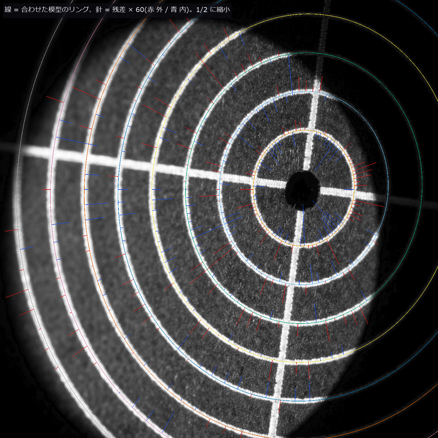
↑ Calibrating an Imaging Model on a Real Telecentric Image — the Scale Matches the Paper, the Entrance Pupil Is Only ‘Farther than 1 m’ ―― An imaging model with plate tilt, orientation, scale, radial distortion k1 and the inverse entrance-pupil distance 1/L (telecentricity) is calibrated with simcal on the ring centrelines of a real 29.5-degree tilted alignment plate (Stark et al., Sci. Rep. 2025, CC BY 4.0). With a noise level independent of the model (local-quadratic pure error, 1.12 px) the absolute chi-square gate fails (p = 7e-9) and the numbers are withdrawn: the 1.35 px residual carries smooth ring-by-ring discrepancy. Adding it as white variance passes all six gates, and only after checking that a ring jackknife agrees with the Laplace uncertainty are numbers reported: 252.14 ± 0.18 px/mm (paper K1 = 252.0) and 1/L = 0.50 ± 0.18 per metre, i.e. the entrance pupil is farther than 1.16 m (2 sigma), which rules out the ordinary f = 100 mm (302 mm) and f = 25 mm lenses. On synthetic data the eight coefficients are recovered at the bound, the ordinary lens’s 1/L = 3.31 per metre within 0.1 sigma of the closed form, an untilted plate makes the orientation ‘no influence’, and a low-order discrepancy makes Laplace 2.4 times optimistic, which the jackknife catches. The 2.7-sigma offset of 1/L from zero is unresolved. No training.
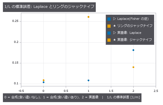
↑ The measurement ―― 【1〜3 章・実画像】入射瞳までの距離の逆数 1/L の標準誤差を 2 通りで出した。Laplace = 白い雑音を仮定したFisher 情報の逆、ジャックナイフ = リングを 1 本ずつ抜いて解き直した散らばり。食い違いの無い合成では2 つは同じ大きさ、リングごとに 0〜6 次の滑らかな食い違い(RMS 0.7 px、リングの半径と中心の癖を含む)を足すと Laplace が 2.4 倍小さく出る(楽観的)。実画像では食い違いを白い分散として足したあと、2 つは同じ大きさ(ジャックナイフ / Laplace = 0.8)—— この板の食い違いは係数の形を真似るほど低次ではない。 (figure labels are in Japanese; the numbers are the same)
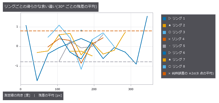
↑ 【実画像】学習の測定線の残差を、リングごと・30° ごとに平均した(点の数は 4 以上)。
py -3.11 examples/poc_simcal_telecentric.py
Source: examples/poc_simcal_telecentric.py
This run produced 3 figures in total - see them all
Ops used (notes): chief_ray_angle · gaussian · project · simcal_discrepancy · simcal_fit · simcal_identifiability · simcal_model · simcal_observe · simcal_screen · simcal_validate · text_box
No.2026.259 —— Deep Scratches Dent the Mean Line — How Much Contamination Robust Gaussian and Spline Filters Survive
Subtracting the waviness before measuring roughness lets a deep scratch pull a linear Gaussian mean line down, so the healthy surface beside it turns into false ridges (2.5 times the true roughness on a profile with 4.3 % scratch samples). The three new roughness ops down-weight the scratch with Tukey’s biweight and iterate, and the mean line stays put (0.97 times). The transfer functions match their closed forms (0.5 at the cutoff; the existing surface_filter gave 0.5095 because of the standard’s literal truncation and was fixed by widening it). The breakdown lies between 35 % and 40 % contamination: at 40 % the mean line is off by 3.5 µm and no better than the linear one. Fixing the weight function to 1 fails the gate, and a non-converging iteration is refused. The truth is closed forms plus a synthetic waviness; no real stylus profile has been checked yet.

↑ Deep Scratches Dent the Mean Line — How Much Contamination Robust Gaussian and Spline Filters Survive ―― Subtracting the waviness before measuring roughness lets a deep scratch pull a linear Gaussian mean line down, so the healthy surface beside it turns into false ridges (2.5 times the true roughness on a profile with 4.3 % scratch samples). The three new roughness ops down-weight the scratch with Tukey’s biweight and iterate, and the mean line stays put (0.97 times). The transfer functions match their closed forms (0.5 at the cutoff; the existing surface_filter gave 0.5095 because of the standard’s literal truncation and was fixed by widening it). The breakdown lies between 35 % and 40 % contamination: at 40 % the mean line is off by 3.5 µm and no better than the linear one. Fixing the weight function to 1 fails the gate, and a non-converging iteration is refused. The truth is closed forms plus a synthetic waviness; no real stylus profile has been checked yet.

↑ The measurement ―― λ = λc = 80 µm でガウス・スプラインとも 0.5。点は閉形式の線の上に乗る(ガウス 1e-7、スプライン 1e-12 の差)。スプラインは遮断が鋭い。 (figure labels are in Japanese; the numbers are the same)

↑ 細い線が傷つき断面。

↑ 線形の引きずりは汚染に比例して増える。
py -3.11 examples/poc_robust_profile_filter.py
Source: examples/poc_robust_profile_filter.py
This run produced 4 figures in total - see them all
Ops used (notes): robust_gaussian_profile · robust_gaussian_surface · robust_spline_profile · surface_filter
No.2026.263 —— Per-Pixel Quadrature Demodulation (Lock-in) — Ring-Illumination Normals, Coded-Light Daylighting and Lock-in Thermography, Scored Against Closed Forms and the Rice Phase Distribution
Per-pixel quadrature demodulation (lock-in) is made a general op on an image sequence, and the three uses of a time-correlation image sensor are shown as variants of one function. Nine new ops (lockin, category lockin of opsoptics): lockin_demodulate (amplitude, phase, DC, in-phase, quadrature and the window leakage), lockin_amplitude, lockin_phase, lockin_noise_floor (closed-form amplitude and phase noise from the SNR), lockin_walsh_codes, lockin_separate (coded lights by least squares), lockin_ring_synthesize, lockin_ring_normals (normals from the first-harmonic response of a multipole-modulated ring) and lockin_thermal_wave (exact surface temperature of a periodically heated plate). A sinusoid of amplitude 2.5, phase 0.7 rad and DC 1.5 is returned to 6.6e-15, and detuning the reference rolls the amplitude off as a sinc (0.4977 at delta-f times T = 0.6033, 0 at 1.0). A length that is not a whole number of periods is refused for the rectangular window; declaring hann returns the leakage in the table (amplitude error 0.0156 at 3.75 periods against a declared bound of 0.0157). With white noise the phase standard deviation at component SNR 45, 11 and 1.7 is 0.0220, 0.0888 and 0.7244 rad measured against 0.0221, 0.0887 and 0.7306 from the closed form of the Rice phase distribution, within 0.9 % (the small-noise approximation is 19 % off at SNR 1.7). (a) Running the phase of an 8-source ring once around the azimuth makes the albedo drop out of the first-harmonic response and leaves the normals: on a surface with an albedo stripe pattern (tilt up to 28.8 degrees) the angle error is 1.0e-13 degrees, and the correlation with the true tilt is -0.035 for the mean image against 1.000000 for the ring normals. The quadrupole reads 0 on a Lambertian surface (3.5e-16). With noise sigma 0.004 the gradient error is 0.0069 measured against 0.0069 predicted (normal-angle RMS 0.56 degrees). A slope beyond the shadow limit is marked invalid instead of given a normal. (b) Three lights switched by Walsh codes are separated to 1.9e-15 even with daylight 2.6 to 4.2 times the lamp, while the best two-frame difference has an error of 0.94 (as large as the lamp image). Under flicker and slow drift the error of lamp 1 is 0.053, 0.031 after a drift column is added, and the flicker shows in the residual image. (c) A 3 mm CFRP plate heated at 0.2 Hz (thermal diffusion length 0.818 mm) has a phase that equals the exact -45 degrees + arg coth((1+j)L/mu) to 1.0e-15, and uneven heating changes the amplitude but not the phase (difference 5.6e-16). The phase standard deviation of the sound area under noise is 0.0213 rad measured against 0.0214 predicted. Voids at 0.3 / 0.6 / 1.0 / 1.5 mm are read from the phase as 0.30 / 0.60 / 1.00 / 1.54 mm (the phase peaks at L/mu = 1.963; deeper voids cannot be read uniquely). Detuning the reference by 10 %, a wrong zenith angle, an undeclared window and dependent codes each turn a gate red or are refused. No learning, no calibration, 25 gates.
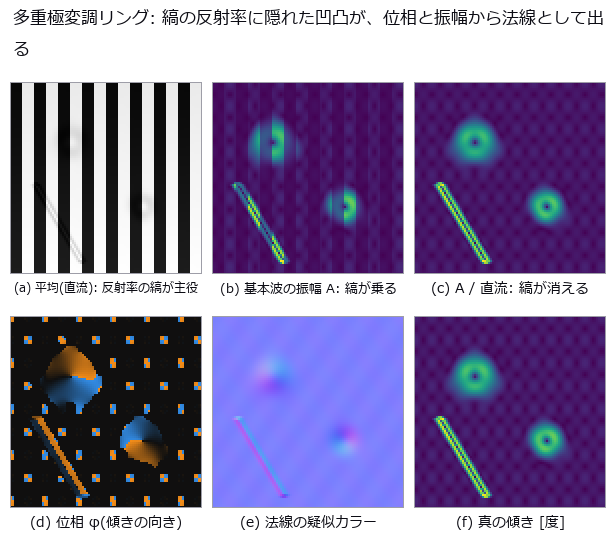
↑ Per-Pixel Quadrature Demodulation (Lock-in) — Ring-Illumination Normals, Coded-Light Daylighting and Lock-in Thermography, Scored Against Closed Forms and the Rice Phase Distribution ―― Per-pixel quadrature demodulation (lock-in) is made a general op on an image sequence, and the three uses of a time-correlation image sensor are shown as variants of one function. Nine new ops (lockin, category lockin of opsoptics): lockin_demodulate (amplitude, phase, DC, in-phase, quadrature and the window leakage), lockin_amplitude, lockin_phase, lockin_noise_floor (closed-form amplitude and phase noise from the SNR), lockin_walsh_codes, lockin_separate (coded lights by least squares), lockin_ring_synthesize, lockin_ring_normals (normals from the first-harmonic response of a multipole-modulated ring) and lockin_thermal_wave (exact surface temperature of a periodically heated plate). A sinusoid of amplitude 2.5, phase 0.7 rad and DC 1.5 is returned to 6.6e-15, and detuning the reference rolls the amplitude off as a sinc (0.4977 at delta-f times T = 0.6033, 0 at 1.0). A length that is not a whole number of periods is refused for the rectangular window; declaring hann returns the leakage in the table (amplitude error 0.0156 at 3.75 periods against a declared bound of 0.0157). With white noise the phase standard deviation at component SNR 45, 11 and 1.7 is 0.0220, 0.0888 and 0.7244 rad measured against 0.0221, 0.0887 and 0.7306 from the closed form of the Rice phase distribution, within 0.9 % (the small-noise approximation is 19 % off at SNR 1.7). (a) Running the phase of an 8-source ring once around the azimuth makes the albedo drop out of the first-harmonic response and leaves the normals: on a surface with an albedo stripe pattern (tilt up to 28.8 degrees) the angle error is 1.0e-13 degrees, and the correlation with the true tilt is -0.035 for the mean image against 1.000000 for the ring normals. The quadrupole reads 0 on a Lambertian surface (3.5e-16). With noise sigma 0.004 the gradient error is 0.0069 measured against 0.0069 predicted (normal-angle RMS 0.56 degrees). A slope beyond the shadow limit is marked invalid instead of given a normal. (b) Three lights switched by Walsh codes are separated to 1.9e-15 even with daylight 2.6 to 4.2 times the lamp, while the best two-frame difference has an error of 0.94 (as large as the lamp image). Under flicker and slow drift the error of lamp 1 is 0.053, 0.031 after a drift column is added, and the flicker shows in the residual image. (c) A 3 mm CFRP plate heated at 0.2 Hz (thermal diffusion length 0.818 mm) has a phase that equals the exact -45 degrees + arg coth((1+j)L/mu) to 1.0e-15, and uneven heating changes the amplitude but not the phase (difference 5.6e-16). The phase standard deviation of the sound area under noise is 0.0213 rad measured against 0.0214 predicted. Voids at 0.3 / 0.6 / 1.0 / 1.5 mm are read from the phase as 0.30 / 0.60 / 1.00 / 1.54 mm (the phase peaks at L/mu = 1.963; deeper voids cannot be read uniquely). Detuning the reference by 10 %, a wrong zenith angle, an undeclared window and dependent codes each turn a gate red or are refused. No learning, no calibration, 25 gates.
Terms: lock-in — A method that correlates with in-phase and quadrature references at a known frequency to recover a periodic signal’s amplitude and phase from broadband noise.
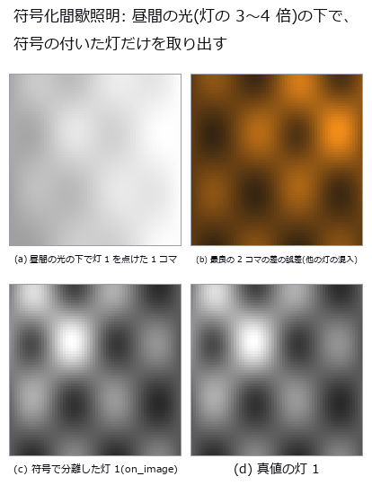
↑ The measurement ―― Walsh 符号 3 本で断続する 3 灯。分離した灯 1 は真値と 1e-12 で一致する。 (figure labels are in Japanese; the numbers are the same)
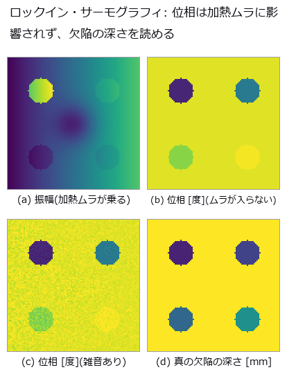
↑ CFRP 板 3 mm、加熱 0.2 Hz(μ = 0.81 mm)。

↑ 周期加熱の熱波が、厚さ L の層の底(断熱面)で反射して表面に戻る遅れ。
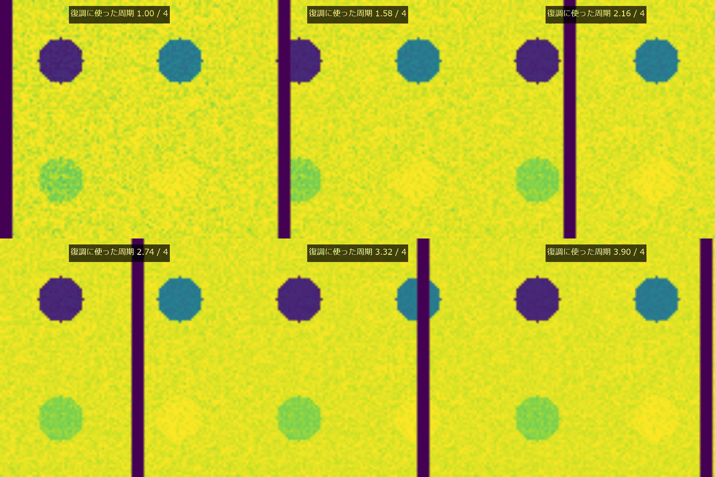
↑ The animation ―― 周期加熱のコマを順に加えると、深さごとの位相像が収束する。
py -3.11 examples/poc_lockin_imaging.py
Source: examples/poc_lockin_imaging.py
This run produced 5 figures in total - see them all
Ops used (notes): lockin_amplitude · lockin_demodulate · lockin_noise_floor · lockin_phase · lockin_ring_normals · lockin_ring_synthesize · lockin_separate · lockin_thermal_wave · lockin_walsh_codes
The Medical and Biological Wing — The Count Is Right and the Contents Are Wrong
Counting cells, reading a nucleus’s DNA content, measuring vessel branching, tracking a wound’s area: all of these tend to be reported as one number, and there are situations in which that number is right anyway. Cell counting where over- and under-segmentation balance to a +0.3-cell bias; ploidy classification that survives a forgotten background subtraction; a calibration that returns the most stable and most wrong healing constant.
The 27 exhibits carry ground truth that a label image alone cannot hold — which cells overlap which, area and DNA content varying independently, a tree that satisfies the branching law exactly. Each docstring warns that calling a label image ‘the truth’ on real data erases the very thing being tested.
The thing to watch for is a method that appears to improve while the quantity it measures quietly swaps: the area classifier gets better with more blur because ‘area’ is leaking DNA content. Unless the reason for every improvement is traced, this kind of lie gets carried home as a result.
No.2026.057 —— Trabecular Thickness, Separation and Bone Volume Fraction — The Plate Model and the Direct Method Disagree on the Same Image
Reported trabecular thickness changes with the definition of truth even on one image. Blur and noise were applied to known-width struts, and distribution overlap was measured at 60 µm pixels. Two biases cancel in the average while the thickness distribution loses agreement as resolution falls.
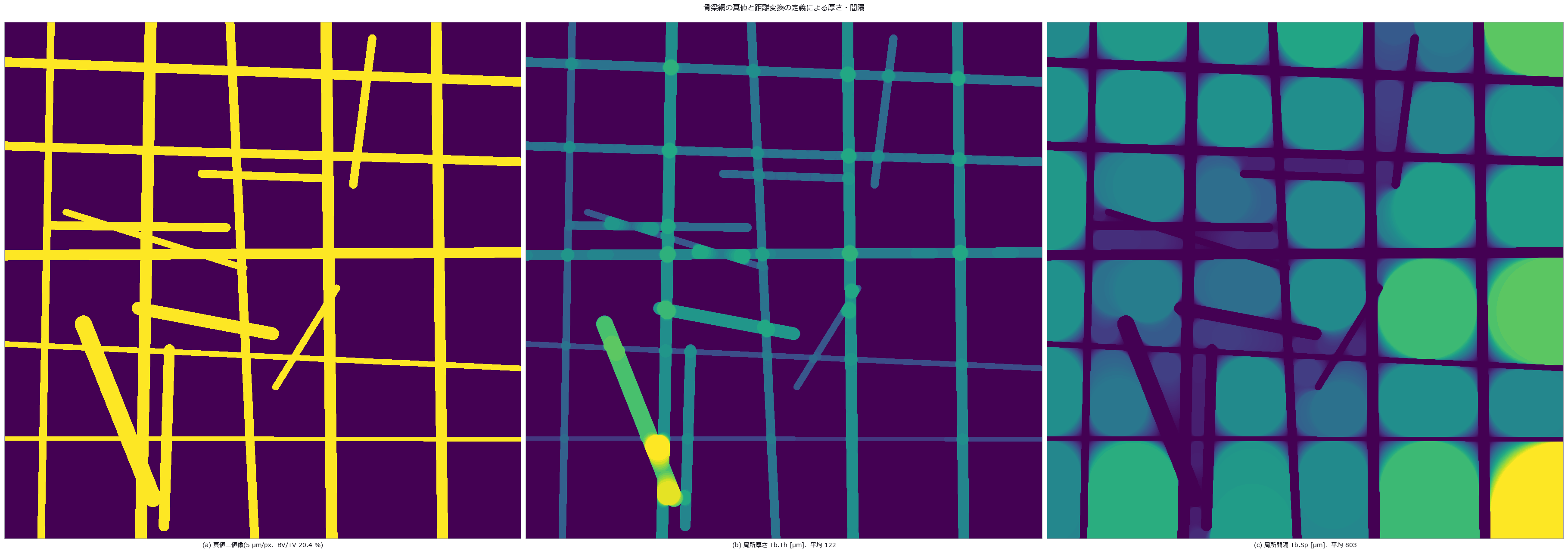
↑ Trabecular Thickness, Separation and Bone Volume Fraction — The Plate Model and the Direct Method Disagree on the Same Image ―― A 2-D trabecular network drawn in closed form as a set of segments (median width 120 µm), observed through partial-volume blur, CT noise and a cupping bias. There is more than one ground truth: the length-weighted mean width is 104.8 µm, the largest-inscribed-circle definition gives 121.6 µm and the plate model 118.4 µm — the choice of truth moves the answer by 9–16 % before any threshold does. The resolution cliff hits the distribution, not the mean (overlap with truth 0.83 → 0.09 at 60 µm pixels; the mean survives because quantisation at -29.5 % and Otsu thickening at +26.6 % cancel). Noise breaks from two sides, speckles from σ 0.10 and gaps from σ 0.15, and an area opening removes only the speckles.
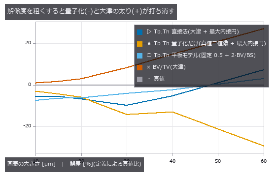
↑ The measurement ―― Tb.Th の平均は 2 px/骨梁でも持つが、BV/TV と分布は壊れている。 (figure labels are in Japanese; the numbers are the same)
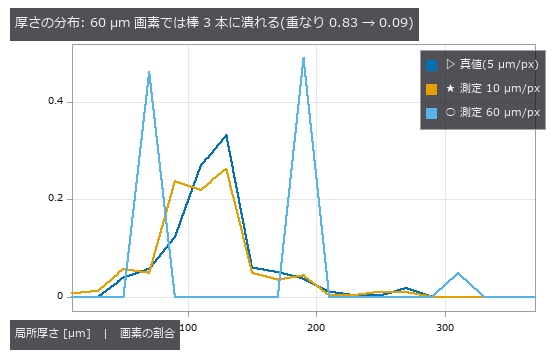
↑ この回の図

↑ この回の図
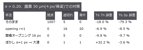
↑ この回の図
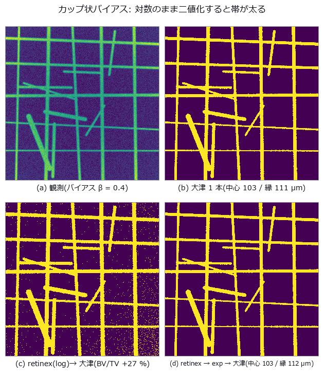
↑ この回の図
py -3.11 examples/poc_bone_trabecular_thickness.py
Source: examples/poc_bone_trabecular_thickness.py
This run produced 14 figures in total - see them all
Ops used (notes): blob_distance · blob_features · blob_label · dc_retinex · dist_transform · gaussian · get_region_thickness · local_thickness · opening_circle · otsu · sk_area_opening · threshold
No.2026.008 —— Counting Overlapping Cells — Count, Over-Segmentation and Under-Segmentation as Three Numbers
Overlapping cells can yield the right total without the right individuals. Overlap was increased in images with known counts, then segmentation was scored on the densest set of 78 cells. Split and merge errors remain where count bias nearly vanishes, so totals cannot select the best setting.
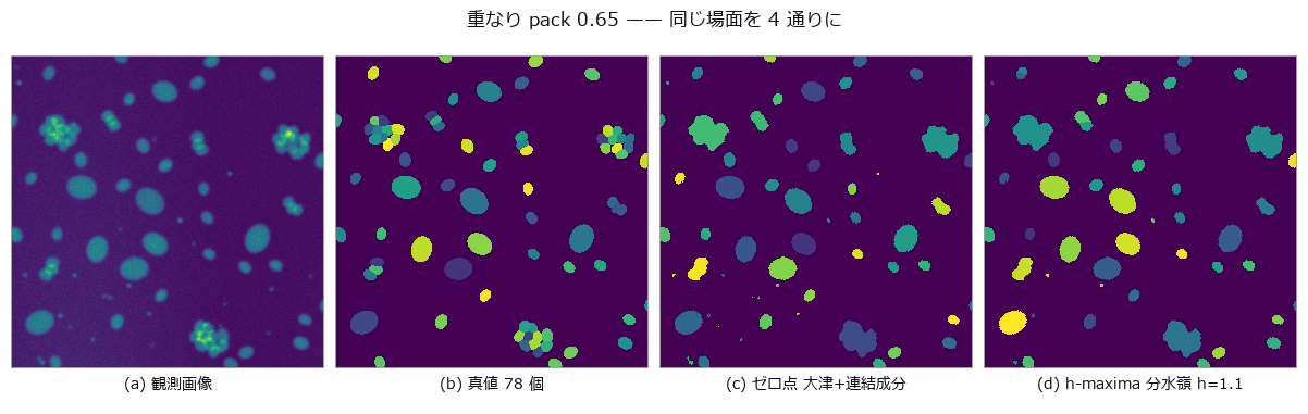
↑ Counting Overlapping Cells — Count, Over-Segmentation and Under-Segmentation as Three Numbers ―― Synthetic overlapping cells with the count, over-segmentation and under-segmentation tallied separately. In the densest condition the null misses 25 of 78 cells, every one of them an under-segmentation. Sweeping the seed suppression finds a balance point where the count bias is +0.3 cells while 13.3 segmentation errors remain; report the count alone and it passes as the best setting.
| [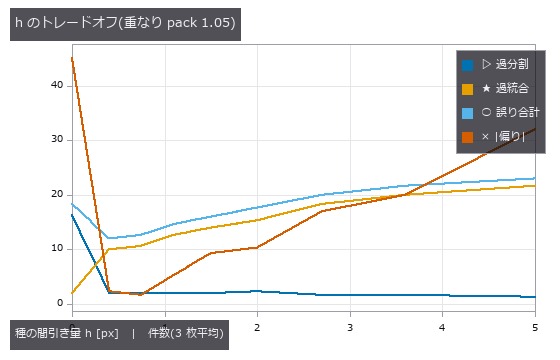](https://raw.githubusercontent.com/furuse-kazufumi/fullseye/master/docs/articles/assets/poc/poc_cell_counting/02_h_tradeoff.png) |
| *↑ The measurement ―― 誤り合計の谷と | 偏り | の谷は同じ場所に来ない。どちらを最適と呼ぶかで答えが変わる。 (figure labels are in Japanese; the numbers are the same)* |
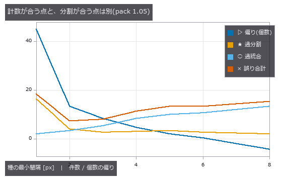
↑ 偏りが 0 を横切る間隔 6 で分割誤りは 13.3 件残る。
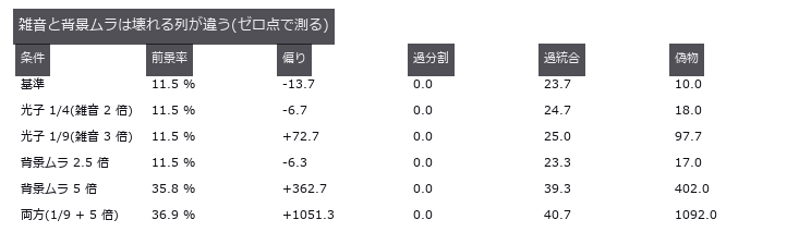
↑ 真値の前景率 11.6 %。
py -3.11 examples/poc_cell_counting.py
Source: examples/poc_cell_counting.py
This run produced 4 figures in total - see them all
Ops used (notes): circularity · distance_transform · fill_holes · gauss_filter · sk_otsu · vol_distance_transform · vol_label · vol_local_maxima · vol_watershed · xsk2_h_maxima
No.2026.061 —— Colocalization lies under bleed-through — Pearson and Manders break in different places
Two channels of vesicle-like puncta are scattered over a synthetic cell body, with 0 / 25 / 50 / 100 % of the B puncta placed exactly on A puncta so the true colocalization is known. After the bleed-through matrix [[1, α], [β, 1]], cytoplasm, PSF and photon noise, two unrelated channels give Pearson r=0.203 and Otsu-Manders M1=0.132 at α=β=10 %. Estimating α=0.0996 (truth 0.10) from single-stain controls and unmixing linearly restores r to 0.007, but Manders stays at 0.699 even for 100 % (the Gaussian tails below the Otsu threshold are lost; closed-form prediction 0.750). Pearson crosses 0.5 at symmetric α=0.282 (predicted 2−√3=0.268); blur only breaks Manders, with a step at σ=2.5 px where Otsu’s foreground jumps from puncta to the whole cell. The Costes shuffle test calls pure bleed-through ‘significant’ at p=0.000.
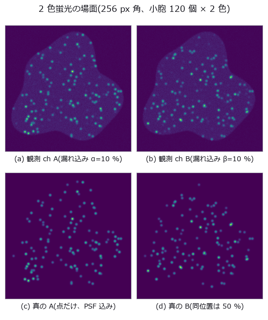
↑ Colocalization lies under bleed-through — Pearson and Manders break in different places ―― Two channels of vesicle-like puncta are scattered over a synthetic cell body, with 0 / 25 / 50 / 100 % of the B puncta placed exactly on A puncta so the true colocalization is known. After the bleed-through matrix [[1, α], [β, 1]], cytoplasm, PSF and photon noise, two unrelated channels give Pearson r=0.203 and Otsu-Manders M1=0.132 at α=β=10 %. Estimating α=0.0996 (truth 0.10) from single-stain controls and unmixing linearly restores r to 0.007, but Manders stays at 0.699 even for 100 % (the Gaussian tails below the Otsu threshold are lost; closed-form prediction 0.750). Pearson crosses 0.5 at symmetric α=0.282 (predicted 2−√3=0.268); blur only breaks Manders, with a step at σ=2.5 px where Otsu’s foreground jumps from puncta to the whole cell. The Costes shuffle test calls pure bleed-through ‘significant’ at p=0.000.
Terms: PSF — The spatial response of an imaging system to a point object, describing how that point is blurred in the image.; Otsu — A histogram thresholding method that chooses the threshold maximizing the variance between the two resulting classes.
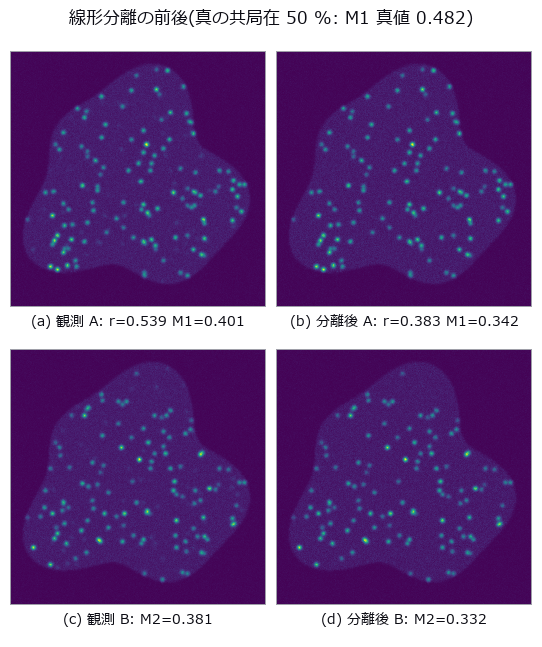
↑ The measurement (figure labels are in Japanese; the numbers are the same)
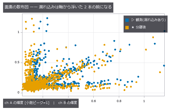
↑ この回の図
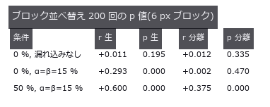
↑ この回の図
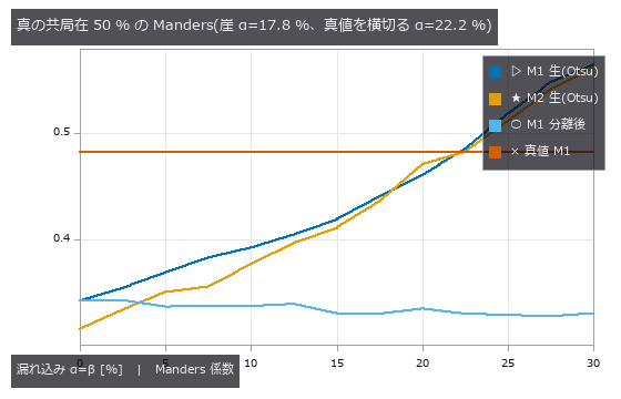
↑ この回の図
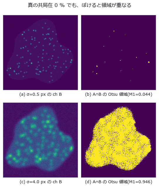
↑ この回の図
py -3.11 examples/poc_colocalization_crosstalk.py
Source: examples/poc_colocalization_crosstalk.py
This run produced 11 figures in total - see them all
Ops used (notes): gauss_image · mat_lstsq · mat_solve · noise_sigma · otsu · photon_sample · reg_erode · stat_correlation
No.2026.074 —— MRI Bias Field and Tissue Area — Grey and White Matter Fail in Opposite Directions, and the Sum Hides It
A brain-slice phantom of elliptical shells (skull / CSF / wrinkled cortex / WM, areas known from geometry) is multiplied by a surface-coil bias field and Rician noise, and the three tissue areas are measured with global three-class Otsu (xsk2_multiotsu). At 30 % amplitude GM is +20.2 % and WM -7.7 % while GM+WM is +0.0 % — the sum hides the error — and removing the noise flips the sign (GM -11.8 %). The geometric cliff prediction was 30 %; the measured cliff is 17.5 %. Naively smoothing log I damages a field-free image by GM +81.8 %; iterating on the segmentation residual (Wells-type) holds +1.8 % even at 40 %. Every corrector fails once the field is as fine as 4 px, and at SNR 15 GM is +8.5 % even without a field (WM is 2.6× larger, so the error lands on the smaller tissue).
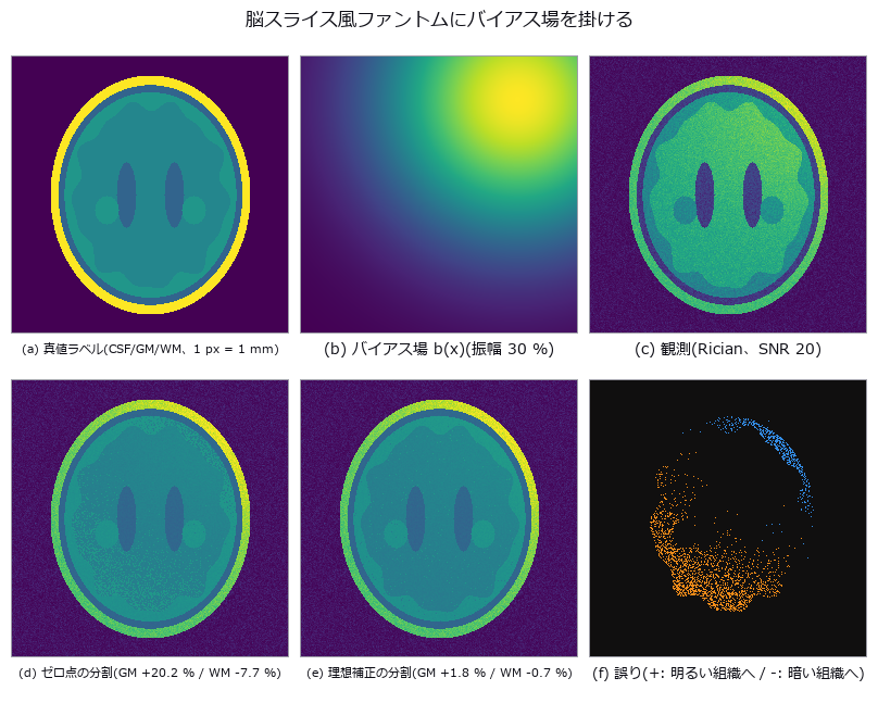
↑ MRI Bias Field and Tissue Area — Grey and White Matter Fail in Opposite Directions, and the Sum Hides It ―― A brain-slice phantom of elliptical shells (skull / CSF / wrinkled cortex / WM, areas known from geometry) is multiplied by a surface-coil bias field and Rician noise, and the three tissue areas are measured with global three-class Otsu (xsk2_multiotsu). At 30 % amplitude GM is +20.2 % and WM -7.7 % while GM+WM is +0.0 % — the sum hides the error — and removing the noise flips the sign (GM -11.8 %). The geometric cliff prediction was 30 %; the measured cliff is 17.5 %. Naively smoothing log I damages a field-free image by GM +81.8 %; iterating on the segmentation residual (Wells-type) holds +1.8 % even at 40 %. Every corrector fails once the field is as fine as 4 px, and at SNR 15 GM is +8.5 % even without a field (WM is 2.6× larger, so the error lands on the smaller tissue).
Terms: Otsu — A histogram thresholding method that chooses the threshold maximizing the variance between the two resulting classes.
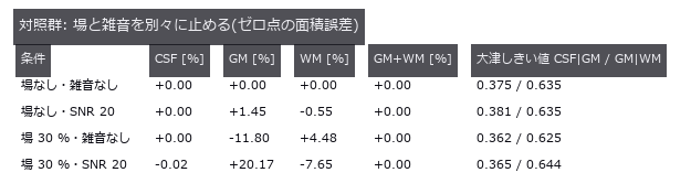
↑ The measurement ―― 雑音だけでは壊れず、場だけで GM と WM が逆向きに動く。 (figure labels are in Japanese; the numbers are the same)

↑ 幾何予測(しきい値固定・雑音なし)と大津の実測は同じ振幅で崖を越える。

↑ この回の図
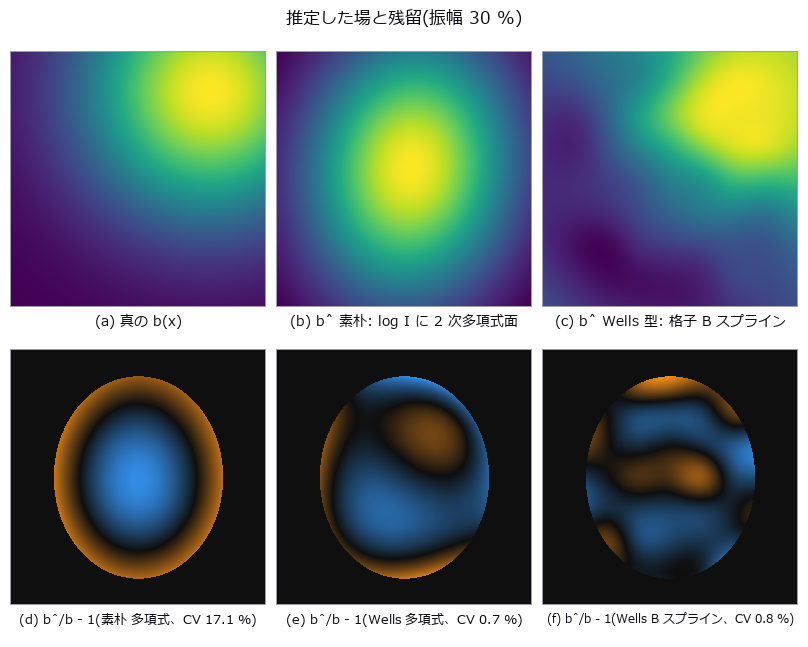
↑ この回の図
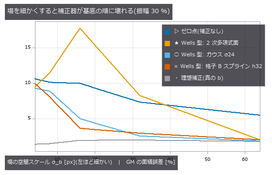
↑ σ_b 4 px は皮質リボンの太さ。
py -3.11 examples/poc_mri_bias_field.py
Source: examples/poc_mri_bias_field.py
This run produced 11 figures in total - see them all
Ops used (notes): dc_homomorphic · eval_bspline_surface · eval_poly_surface · fit_bspline_surface · fit_poly_surface · overlay_labels · xsk2_multiotsu
No.2026.027 —— Ploidy From Integrated Nuclear Intensity — Area Cannot Separate It
Fluorescent nuclei whose DNA content D and area A were drawn with independent spread, classified by area and by integrated intensity. Even the true area misclassifies 15.4 %; integrated intensity misclassifies 0 %. Forgetting to subtract background leaves the classification intact while the DNA index alone breaks from 2.115 to 1.702 (-20 %) — invisible if you only watch the classification.
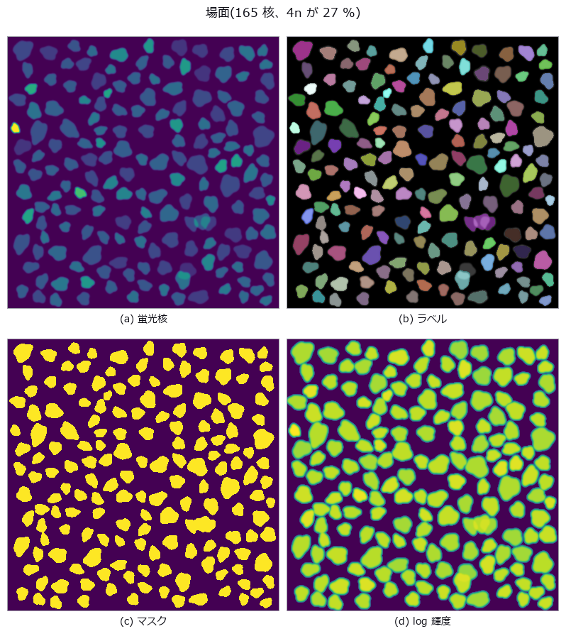
↑ Ploidy From Integrated Nuclear Intensity — Area Cannot Separate It ―― Fluorescent nuclei whose DNA content D and area A were drawn with independent spread, classified by area and by integrated intensity. Even the true area misclassifies 15.4 %; integrated intensity misclassifies 0 %. Forgetting to subtract background leaves the classification intact while the DNA index alone breaks from 2.115 to 1.702 (-20 %) — invisible if you only watch the classification.
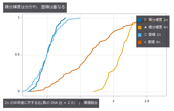
↑ The measurement ―― 累積分布。積分輝度の 4n は 2.1 付近に固まり、面積の 2 本は大きく重なる。 (figure labels are in Japanese; the numbers are the same)
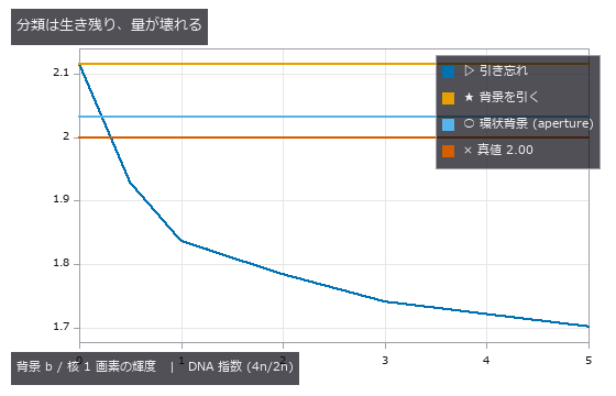
↑ 誤分類率はほぼ 0 のままだが、DNA 指数は背景とともに 2.00 から落ちる。
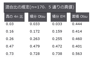
↑ 特徴量が分かれてさえいれば割り方は選ばない。
py -3.11 examples/poc_nuclei_ploidy.py
Source: examples/poc_nuclei_ploidy.py
This run produced 4 figures in total - see them all
Ops used (notes): aperture_photometry · blob_features · blob_label · blob_overlay · gaussian · median · sg_gmm_segment · sk_otsu
No.2026.048 —— Extracting a Vessel Network — Spurs, Overestimated Radii Near Branches, and a Fragile Exponent
A synthetic vessel tree obeying Murray’s law exactly, skeletonised and measured for branch points, radii and the exponent. Counting branch pixels directly gives 47 pixels for 25 branches; grouping them into connected components gives exactly 25. Spurs come not from the skeletonisation but from boundary roughness (spurious branches 0 → 72), and radii within 3 px of a branch are overestimated by +26.2 %.
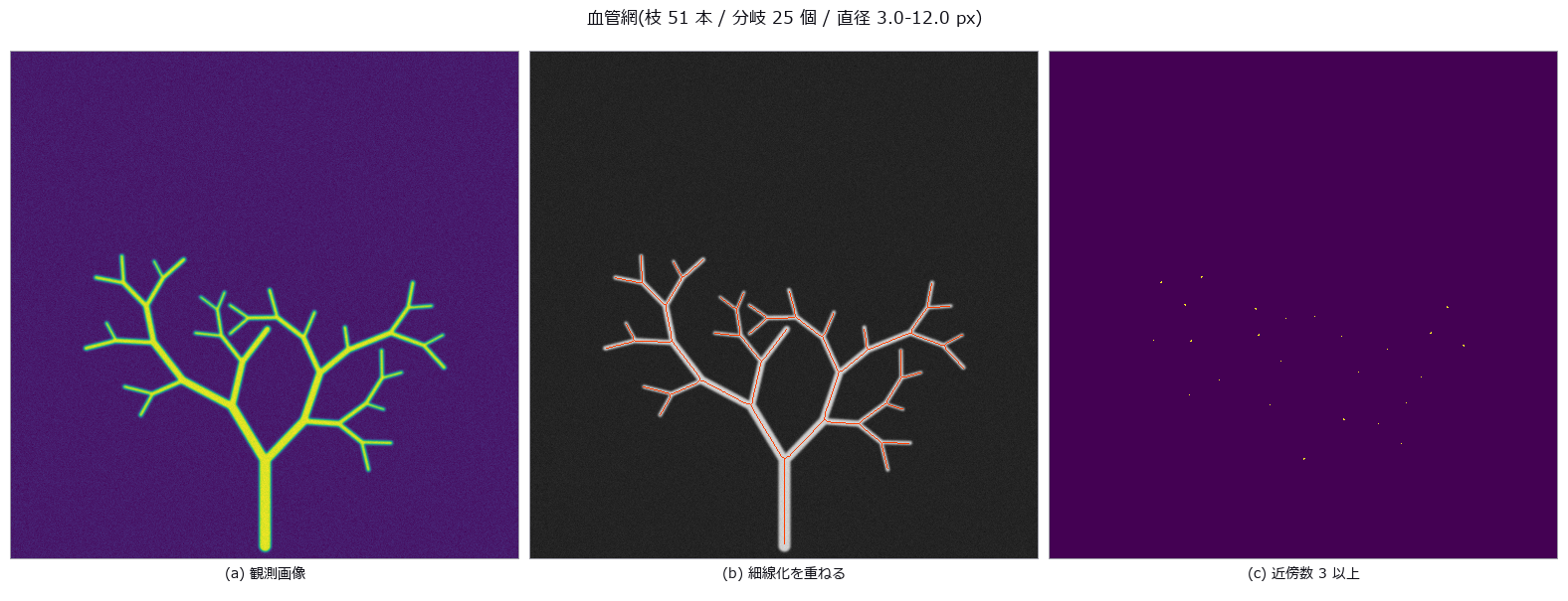
↑ Extracting a Vessel Network — Spurs, Overestimated Radii Near Branches, and a Fragile Exponent ―― A synthetic vessel tree obeying Murray’s law exactly, skeletonised and measured for branch points, radii and the exponent. Counting branch pixels directly gives 47 pixels for 25 branches; grouping them into connected components gives exactly 25. Spurs come not from the skeletonisation but from boundary roughness (spurious branches 0 → 72), and radii within 3 px of a branch are overestimated by +26.2 %.
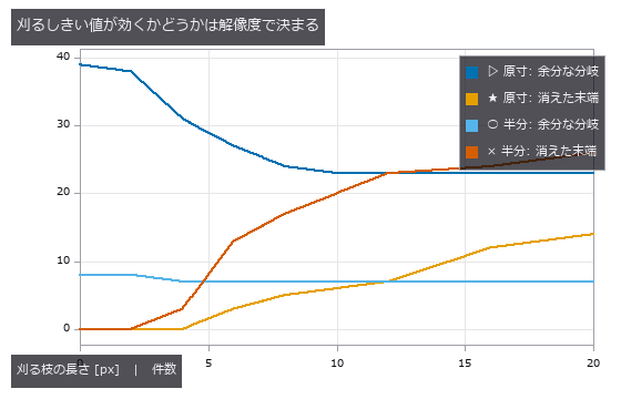
↑ The measurement (figure labels are in Japanese; the numbers are the same)
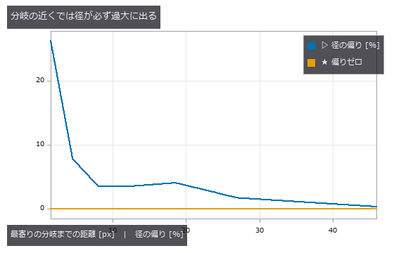
↑ この回の図
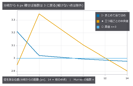
↑ 分岐から 2 px の点は 1 つも解けなかったので図から外した
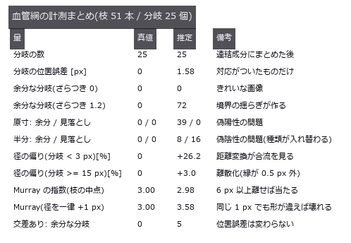
↑ この回の図
py -3.11 examples/poc_vessel_network.py
Source: examples/poc_vessel_network.py
This run produced 5 figures in total - see them all
Ops used (notes): blob_features · blob_label · distance_transform · gauss_filter · medial_axis_points · r2_split_skeleton_lines · sk_medial · skeleton · skeleton_branches3d · skeleton_endpoints3d · skeleton_junctions3d · skeleton_prune3d · skeletonize_vol · thinning · vol_distance_transform
No.2026.052 —— Wound Area Over Time — Calibration Error Enters the Area Squared
A star-shaped wound on a millimetre plane (closed-form area), photographed day by day through a pinhole camera to estimate the healing constant k. A 4 % change in distance moves the area by 7.7 %; with the distance drifting 1.2 % per day the null reports k = 0.1424 against a true 0.1200 (+18.7 %). Its standard deviation, 0.0049, is smaller than the 0.0059 of recalibrating every time — the most stable and the most wrong answer.
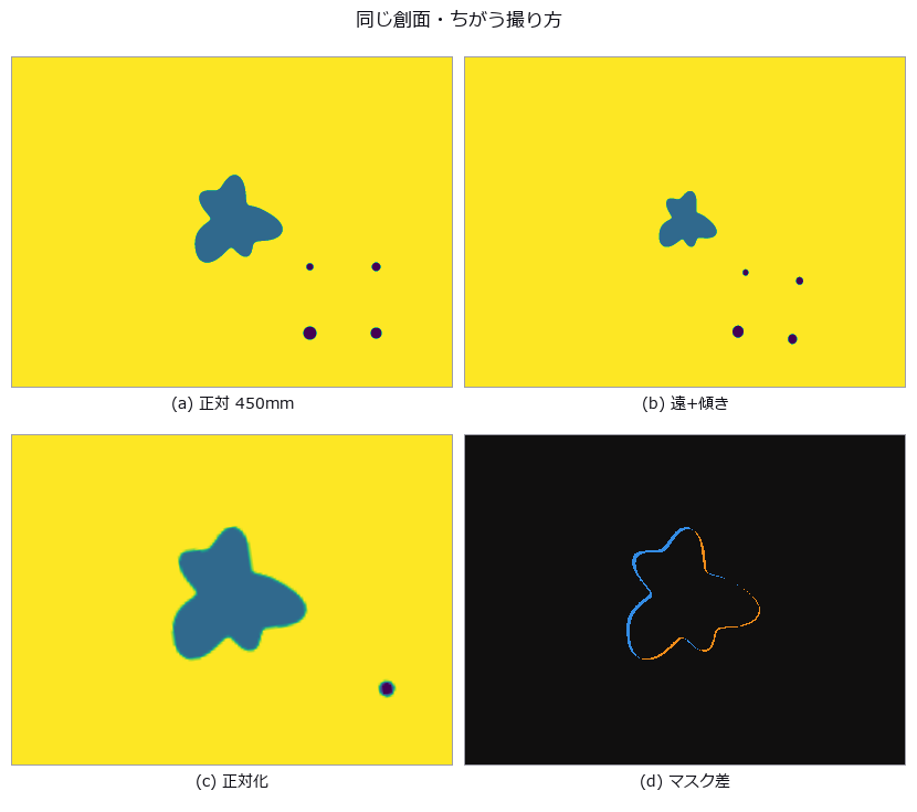
↑ Wound Area Over Time — Calibration Error Enters the Area Squared ―― A star-shaped wound on a millimetre plane (closed-form area), photographed day by day through a pinhole camera to estimate the healing constant k. A 4 % change in distance moves the area by 7.7 %; with the distance drifting 1.2 % per day the null reports k = 0.1424 against a true 0.1200 (+18.7 %). Its standard deviation, 0.0049, is smaller than the 0.0059 of recalibrating every time — the most stable and the most wrong answer.

↑ The measurement ―― ゼロ点の面積誤差。実測は閉形式の 2 乗則に乗り、線形近似からは外れる。 (figure labels are in Japanese; the numbers are the same)
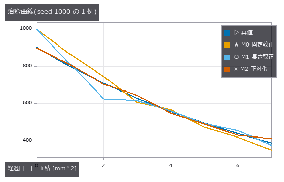
↑ ゼロ点は毎回もっともらしい値を返しながら、傾きだけが系統的に急になる。
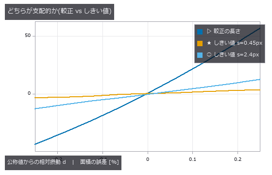
↑ 較正は d に対して (1+d)²-1、しきい値はほぼ線形。
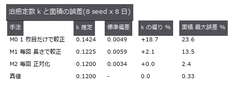
↑ ゼロ点は散らばりがいちばん小さく、偏りがいちばん大きい。
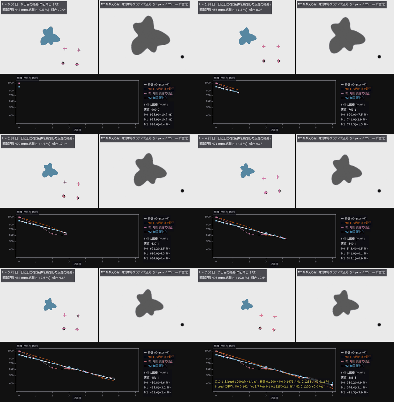
↑ The animation ―― 動画(800 × 544、12 fps、143 コマ): 真の面積 A0·exp(-kt)(k = 0.12 /day)で縮む創面を 8 日撮る。撮影距離は 1 日 +1.2 % 漂い(この 1 本では 448 → 495 mm)、傾き・方位・回転も毎回変わる(日と日の間は条件を補間した仮想の撮影、整数日のコマが門と同じ 1 枚)。左 = カメラの像(水色 = 測った塊、紫の十字 = 較正標識)、右 = 正対化した像。M0(1 枚目だけで較正)は0 日目 +10.7 % から 7 日目 -9.9 % へ真値の下へ漂い、下の対数グラフで M0 の傾きだけが急になる。この 1 本の k は M0 0.1473 / M1 0.1253 / M2 0.1174(真値 0.1200)、8 seed の平均は M0 0.1424(+18.7 %)/ M1 0.1225(+2.1 %)/ M2 0.1200(+0.0 %)。
py -3.11 examples/poc_wound_area_tracking.py
Source: examples/poc_wound_area_tracking.py
This run produced 6 figures in total - see them all
Ops used (notes): axes_frame · axes_transform · blob_features · blob_label · blob_select_largest · contour_to_world_plane_xld · data_to_pixel · gaussian · hom_vector_to_proj_hom_mat2d · image_to_world_plane · plot_series · text_box · ticks · warp_by_plane
No.2026.123 —— A Larval Connectome as a Reservoir Reads Digits — and the Wiring Is Not What Does It
The complete larval Drosophila connectome (Winding 2023: 2,952 neurons, 110,677 edges) used as a fixed recurrent network with only a closed-form ridge readout reads an MNIST subset (4,000 train, 1,000 test) at 91.9 % (ridge on raw pixels: 77.6 %). Prior work stops there; this exhibit adds the controls: a graph with every neuron’s in- and out-degree preserved but the edges rewired reaches 91.6 %, a random graph of the same density 91.9 %, a Gaussian random reservoir 91.5 %. The gap is +0.3 points over 3 seeds. What the readout uses is the reservoir as a mechanism, not the wiring evolution chose. The setting (input scale and regularisation) is chosen once on the connectome’s validation split and reused for every control.

↑ A Larval Connectome as a Reservoir Reads Digits — and the Wiring Is Not What Does It ―― The complete larval Drosophila connectome (Winding 2023: 2,952 neurons, 110,677 edges) used as a fixed recurrent network with only a closed-form ridge readout reads an MNIST subset (4,000 train, 1,000 test) at 91.9 % (ridge on raw pixels: 77.6 %). Prior work stops there; this exhibit adds the controls: a graph with every neuron’s in- and out-degree preserved but the edges rewired reaches 91.6 %, a random graph of the same density 91.9 %, a Gaussian random reservoir 91.5 %. The gap is +0.3 points over 3 seeds. What the readout uses is the reservoir as a mechanism, not the wiring evolution chose. The setting (input scale and regularisation) is chosen once on the connectome’s validation split and reused for every control.
| [](https://raw.githubusercontent.com/furuse-kazufumi/fullseye/master/docs/articles/assets/poc/poc_larval_connectome_reservoir/02_activity_raster_connectome_vs_shuffle.png) |
| *↑ The measurement ―― | state | of the 300 highest-degree neurons over 6 steps for one test digit: connectome | shuffle (figure labels are in Japanese; the numbers are the same)* |

↑ test accuracy per reservoir variant (rows: no reservoir, connectome, shuffle, ER, Gaussian)
py -3.11 examples/poc_larval_connectome_reservoir.py
Source: examples/poc_larval_connectome_reservoir.py
This run produced 3 figures in total - see them all
Ops used (notes): graph_degree_preserving_shuffle · graph_degree_table · graph_spectral_radius · reservoir_encode · reservoir_from_graph · ridge_predict · ridge_readout
No.2026.124 —— Watching a Pulse Travel the Wiring on the 3-D Fly Brain — Connectome vs Degree-Preserving Shuffle
| The previous exhibit ended with ‘readout accuracy cannot tell the connectome from a random graph’. This one uses the same reservoir to look: the 3,000 somatic neurons of the MaleCNS with the most synapses (344,719 edges) receive a pulse into the right optic lobe only, and the activity is drawn on the rotating 3-D brain and VNC (grey = all 141,781 somata, orange = right, blue = left). Next to it, a graph with every neuron’s in- and out-degree preserved but the edges rewired gets the same pulse through the same input matrix. Measured: in the connectome the | x | -weighted mean distance from the stimulus grows 88 → 230 µm over 17 steps, and neurons light in order optic (latency 0) → central (2) → descending (2), never reaching the VNC within 36 steps. In the shuffle the activity scatters to 300 µm in 3 steps and 93 % of the farthest quarter of the neurons light within the first period (connectome: 0 %). The spatial structure of the wiring that accuracy could not see is visible in motion. One brightness scale for every frame. Besides the rotating view, a second animation shows the same instant from three fixed directions at once (dorsal, lateral, along the body axis; views=). Raw data is never committed (the subgraph is built from local feather files and cached; without them a distance-wired synthetic surrogate runs the same path). |
| ↑ Watching a Pulse Travel the Wiring on the 3-D Fly Brain — Connectome vs Degree-Preserving Shuffle ―― The previous exhibit ended with ‘readout accuracy cannot tell the connectome from a random graph’. This one uses the same reservoir to *look: the 3,000 somatic neurons of the MaleCNS with the most synapses (344,719 edges) receive a pulse into the right optic lobe only, and the activity is drawn on the rotating 3-D brain and VNC (grey = all 141,781 somata, orange = right, blue = left). Next to it, a graph with every neuron’s in- and out-degree preserved but the edges rewired gets the same pulse through the same input matrix. Measured: in the connectome the | x | -weighted mean distance from the stimulus grows 88 → 230 µm over 17 steps, and neurons light in order optic (latency 0) → central (2) → descending (2), never reaching the VNC within 36 steps. In the shuffle the activity scatters to 300 µm in 3 steps and 93 % of the farthest quarter of the neurons light within the first period (connectome: 0 %). The spatial structure of the wiring that accuracy could not see is visible in motion. One brightness scale for every frame. Besides the rotating view, a second animation shows the same instant from three fixed directions at once (dorsal, lateral, along the body axis; views=). Raw data is never committed (the subgraph is built from local feather files and cached; without them a distance-wired synthetic surrogate runs the same path).* |
↑ The measurement ―― a pulse into the right optic lobe (orange = right, blue = left somata; grey = all 141781 somata) propagates through the real wiring (left) and through the same degrees rewired at random (right); 3000 neurons, 344719 edges, 36 steps, one brightness scale for every frame (figure labels are in Japanese; the numbers are the same)
| *↑ when each neuron first lights up (yellow = step 0, orange = step 3, blue = step 6 or later, grey = never within 36 steps): connectome | shuffle* |
| [](https://raw.githubusercontent.com/furuse-kazufumi/fullseye/master/docs/articles/assets/poc/poc_malecns_activity_wave/04_activity_spread_mean_distance.png) |
| *↑ graph_activity_spread: | x | -weighted mean distance from the stimulated somata* |
py -3.11 examples/poc_malecns_activity_wave.py
Source: examples/poc_malecns_activity_wave.py
This run produced 4 figures in total - see them all
Ops used (notes): graph_activation_latency · graph_activity_spread · graph_degree_preserving_shuffle · points_activity_video · reservoir_from_graph · reservoir_states · text_box
No.2026.125 —— What the Compound Eye Sees, and Where the Brain Answers — Trace an Ommatidium and the Response Travels the Wiring
The MaleCNS annotations give every optic-lobe neuron a hexagonal column (the column that belongs to one ommatidium of the retina). The 892 right-eye columns (top 3 neurons each) plus 1,400 central and descending hubs form a subgraph of 4,076 neurons and 150,487 edges, stimulated at the resolution of a single ommatidium. Animation 1: as the stimulated column moves along a row of the eye, the response (yellow = stimulated, orange = right, blue = left; scale = response peak excluding the stimulus) moves the same way inside the optic lobe — the correlation between the stimulated column and the response centroid is −0.92 for the connectome and +0.01 for the degree-preserving shuffle with the same input matrix. Retinotopy lives in the wiring and not in the degrees. Animation 2: a bar crossing the visual field is resampled onto the ommatidial lattice (fly_hex_resample) and each ommatidium’s brightness drives its column; the response follows the bar (dorsal and lateral views). In Studio, Tools ▸ Compound eye → brain runs the same parts interactively: hover to stimulate the column under the mouse, drag to orbit, feed the current Studio image through the eye, switch to the shuffle. The column-to-ommatidium mapping is an approximation by normalised hexagonal coordinates. Neither the raw data nor the subgraph is committed (cached from local feather files; without them a synthetic surrogate with hexagonal columns runs the same path).
↑ What the Compound Eye Sees, and Where the Brain Answers — Trace an Ommatidium and the Response Travels the Wiring ―― The MaleCNS annotations give every optic-lobe neuron a hexagonal column (the column that belongs to one ommatidium of the retina). The 892 right-eye columns (top 3 neurons each) plus 1,400 central and descending hubs form a subgraph of 4,076 neurons and 150,487 edges, stimulated at the resolution of a single ommatidium. Animation 1: as the stimulated column moves along a row of the eye, the response (yellow = stimulated, orange = right, blue = left; scale = response peak excluding the stimulus) moves the same way inside the optic lobe — the correlation between the stimulated column and the response centroid is −0.92 for the connectome and +0.01 for the degree-preserving shuffle with the same input matrix. Retinotopy lives in the wiring and not in the degrees. Animation 2: a bar crossing the visual field is resampled onto the ommatidial lattice (fly_hex_resample) and each ommatidium’s brightness drives its column; the response follows the bar (dorsal and lateral views). In Studio, Tools ▸ Compound eye → brain runs the same parts interactively: hover to stimulate the column under the mouse, drag to orbit, feed the current Studio image through the eye, switch to the shuffle. The column-to-ommatidium mapping is an approximation by normalised hexagonal coordinates. Neither the raw data nor the subgraph is committed (cached from local feather files; without them a synthetic surrogate with hexagonal columns runs the same path).
↑ The measurement ―― a stimulus of one eye column (+ its 6 neighbours) moves along a row of the right eye; yellow = stimulated neurons, orange/blue = response (scale = response peak); the connectome answers retinotopically, the shuffle does not (figure labels are in Japanese; the numbers are the same)
| [](https://raw.githubusercontent.com/furuse-kazufumi/fullseye/master/docs/articles/assets/poc/poc_eye_to_brain/03_retinotopy_scatter.png) |
| *↑ | x | -weighted centroid of the responding optic-lobe neurons vs the stimulated column* |

↑ fly_hex_quantize(mode=log): a low-contrast soft bar (0.5 + 0.3, sigma 6 px) crossing the visual field is quantized to n bits per ommatidium before ent…
py -3.11 examples/poc_eye_to_brain.py
Source: examples/poc_eye_to_brain.py
This run produced 4 figures in total - see them all
Ops used (notes): fly_hex_quantize · points_activity_video · text_box
No.2026.126 —— A Second Opinion for EM Connectome Proofreading — Membranes Belong Only on Label Boundaries
Automatic segmentation of serial EM sections leaves merges (two cells under one id) and splits (one cell under two ids); every prior detector is a deep network. This PoC counts the same two errors without learning, from one premise read two ways — a cell membrane (dark ridge) belongs only on label boundaries: a membrane chord crossing the inside of a label = merge suspect (closed rings, i.e. mitochondria, are excluded by their hole), a boundary without membrane = split suspect. Artificial merges and splits are injected into the ground-truth labels of CREMI sample A (12 slices of 512², raw data never committed); with thresholds chosen on the first 6 slices and every number reported on the last 6, splits reach AUC 1.00 (TPR 1.00 / FPR 0.11) and merges AUC 0.83 against area-matched negatives (TPR 0.12 / FPR 0.01; random 0.53, area only 0.70). Merge detection is weak: membrane-rich cells score like chords. Because an injected merge is the union of two large labels, measuring without area matching yields 0.87 from ‘big label = suspicious’ alone — the reason holdout_threshold, which separates the slices that choose the threshold from the slices that are measured, is an operator. The animation rotates the stacked cube with suspects on top (magenta = merge, cyan = split, brightness = score). New family emproof (7 ops, numpy + scipy only).
↑ A Second Opinion for EM Connectome Proofreading — Membranes Belong Only on Label Boundaries ―― Automatic segmentation of serial EM sections leaves merges (two cells under one id) and splits (one cell under two ids); every prior detector is a deep network. This PoC counts the same two errors without learning, from one premise read two ways — a cell membrane (dark ridge) belongs only on label boundaries: a membrane chord crossing the inside of a label = merge suspect (closed rings, i.e. mitochondria, are excluded by their hole), a boundary without membrane = split suspect. Artificial merges and splits are injected into the ground-truth labels of CREMI sample A (12 slices of 512², raw data never committed); with thresholds chosen on the first 6 slices and every number reported on the last 6, splits reach AUC 1.00 (TPR 1.00 / FPR 0.11) and merges AUC 0.83 against area-matched negatives (TPR 0.12 / FPR 0.01; random 0.53, area only 0.70). Merge detection is weak: membrane-rich cells score like chords. Because an injected merge is the union of two large labels, measuring without area matching yields 0.87 from ‘big label = suspicious’ alone — the reason holdout_threshold, which separates the slices that choose the threshold from the slices that are measured, is an operator. The animation rotates the stacked cube with suspects on top (magenta = merge, cyan = split, brightness = score). New family emproof (7 ops, numpy + scipy only).
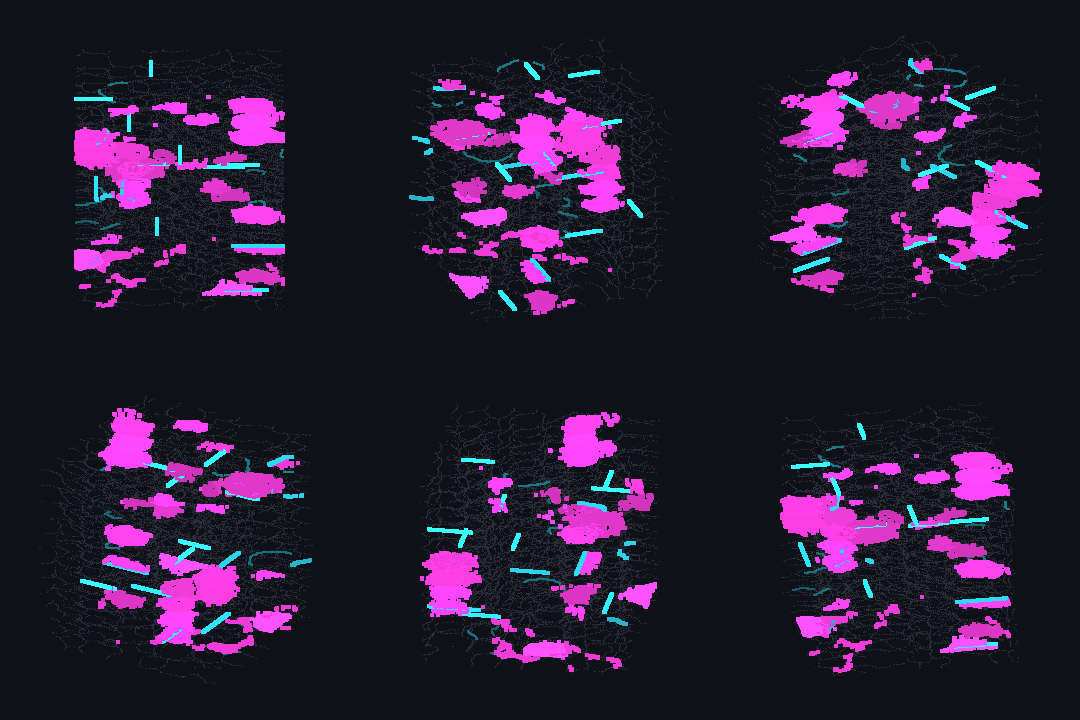
↑ The measurement ―― suspects on the stacked cube: magenta = merge suspects (membrane chords), cyan = split suspects (membrane-free boundaries), brightness = score, grey = all label boundaries (figure labels are in Japanese; the numbers are the same)
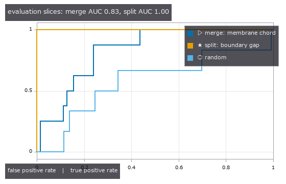
↑ ROC on the held-out slices; thresholds were chosen on the other half
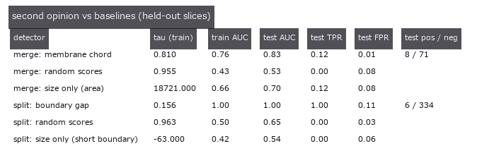
↑ tau = smallest threshold with train FPR <= 5 %; every number in the test columns comes from slices the threshold never saw
py -3.11 examples/poc_em_second_opinion.py
Source: examples/poc_em_second_opinion.py
This run produced 4 figures in total - see them all
Ops used (notes): holdout_threshold · points_activity_video · seg_boundary_membrane_gap · seg_inject_merge · seg_inject_split · seg_label_changes · seg_membrane_chord_score · seg_membrane_response
No.2026.129 —— Motor Quantisation — Where the Command Dimension Collapses Between Brain and Muscle (the Fly’s Neck and an RL Policy’s Joints on One Scale)
You do not think about individual muscles when you raise an arm: the tens of thousands of brain states must be folded into a few commands somewhere, and in the fly that somewhere is visible in the wiring — MaleCNS v1.0 (Janelia, CC BY 4.0): 32,164 central-brain interneurons → the narrow neck of 1,314 descending neurons (DN) → 13,161 nerve-cord interneurons → 708 motor neurons (MN). With four ops added to conngraph (graph_layer_propagate / graph_block_shuffle / states_participation_ratio / states_layer_dimension) the brain → DN → VNC → MN subgraph (4,022 neurons) is driven by 400 random sparse stimuli and the effective dimension of each layer’s states (participation ratio, Gao et al. 2017) is read. With sparse firing (kWTA 10 %) it falls monotonically 282 > 61 > 8.7 > 2.4; picking 708 columns of the brain states still gives 249, so the fall is not the layer size. A control that keeps every receiver’s input weights but shuffles who sends them leaves the MN at 21.9 — the VNC → muscle stage compresses by the specific wiring, while the neck (DN) stage matches the control (61 vs 62) and compresses by convergence alone. Honest breakdown: the raw PR is also pulled by a heavy tail (a few stimuli drive the MN 17× harder than the median), so the direction-only dimension (every response scaled to unit norm) was measured too — real wiring 25 vs control 54 (kWTA), 7 vs 42 (linear). The same formula on Physical AI: joint trajectories of a humanoid robot’s RL walking and running score 1.5–4.1 (median 3.2), dance 9.3, fight 11.9, and evis muscle activations (up to 73 muscles) 5.8–9.6. An order-of-magnitude comparison, not a claim of identity. Raw data and subgraphs are never committed.
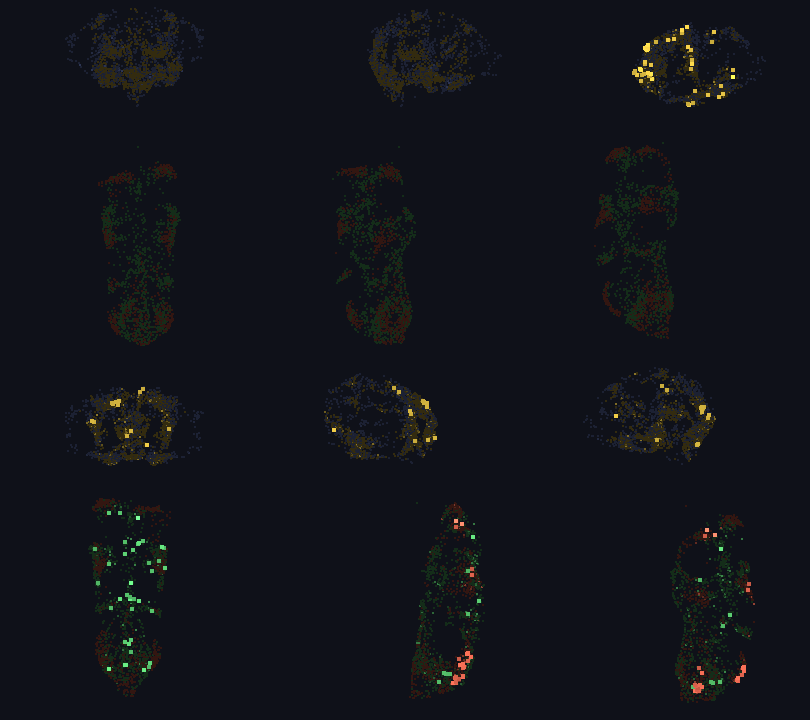
↑ Motor Quantisation — Where the Command Dimension Collapses Between Brain and Muscle (the Fly’s Neck and an RL Policy’s Joints on One Scale) ―― You do not think about individual muscles when you raise an arm: the tens of thousands of brain states must be folded into a few commands somewhere, and in the fly that somewhere is visible in the wiring — MaleCNS v1.0 (Janelia, CC BY 4.0): 32,164 central-brain interneurons → the narrow neck of 1,314 descending neurons (DN) → 13,161 nerve-cord interneurons → 708 motor neurons (MN). With four ops added to conngraph (graph_layer_propagate / graph_block_shuffle / states_participation_ratio / states_layer_dimension) the brain → DN → VNC → MN subgraph (4,022 neurons) is driven by 400 random sparse stimuli and the effective dimension of each layer’s states (participation ratio, Gao et al. 2017) is read. With sparse firing (kWTA 10 %) it falls monotonically 282 > 61 > 8.7 > 2.4; picking 708 columns of the brain states still gives 249, so the fall is not the layer size. A control that keeps every receiver’s input weights but shuffles who sends them leaves the MN at 21.9 — the VNC → muscle stage compresses by the specific wiring, while the neck (DN) stage matches the control (61 vs 62) and compresses by convergence alone. Honest breakdown: the raw PR is also pulled by a heavy tail (a few stimuli drive the MN 17× harder than the median), so the direction-only dimension (every response scaled to unit norm) was measured too — real wiring 25 vs control 54 (kWTA), 7 vs 42 (linear). The same formula on Physical AI: joint trajectories of a humanoid robot’s RL walking and running score 1.5–4.1 (median 3.2), dance 9.3, fight 11.9, and evis muscle activations (up to 73 muscles) 5.8–9.6. An order-of-magnitude comparison, not a claim of identity. Raw data and subgraphs are never committed.
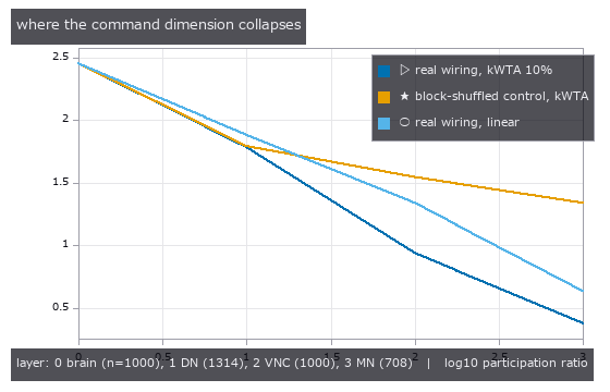
↑ The measurement ―― effective dimension of the states each layer takes under 400 random sparse stimuli of the brain layer: real wiring vs a control that keeps every receiver’s input weights but shuffles who sends them; the neck (DN) compresses by convergence alone, the VNC -> MN stage compresses by the specific wiring (figure labels are in Japanese; the numbers are the same)

↑ the same funnel after every stimulus response is scaled to unit norm (magnitude removed, direction kept): the real wiring still leaves fewer MN direct…

↑ the 400 stimuli projected on the first two principal components of the MN states: real wiring folds them onto a few directions, the shuffled control s…

↑ participation ratio of joint-angle trajectories (a humanoid robot, RL policies and mocap retargets), next to the fly’s MN command dimension (2.4) unde…
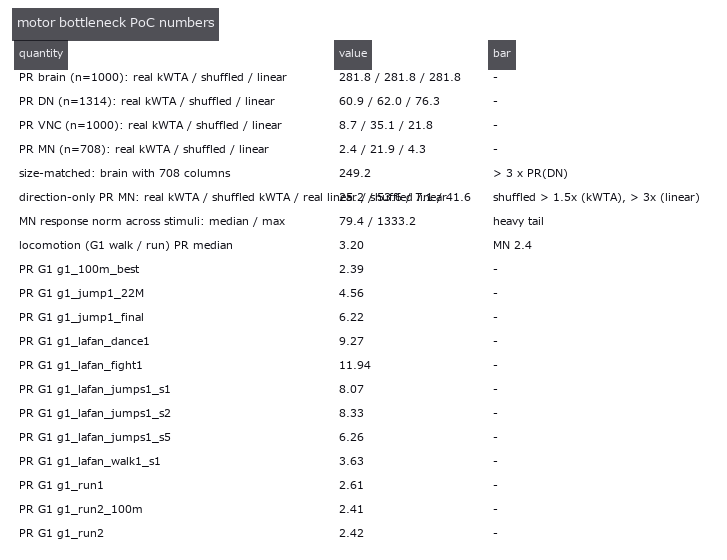
↑ every number, with the bar it had to clear
py -3.11 examples/poc_connectome_motor_bottleneck.py
Source: examples/poc_connectome_motor_bottleneck.py
This run produced 6 figures in total - see them all
Ops used (notes): graph_block_shuffle · graph_layer_propagate · points_activity_video · states_layer_dimension · states_participation_ratio
No.2026.131 —— The MICrONS Brain Wave — How Much of the Measured Response Does the Wiring Explain in 1 mm^3 of Visual Cortex
MICrONS (about 1 mm^3 of mouse V1 plus higher visual areas) is the rare dataset that holds both the electron-microscopy wiring and the two-photon activity of the same neurons. The public tables of Ding et al. 2025 (Nature) — 12,894 neurons with soma position, visual area and a 120-frame trial-averaged response to a natural movie, and 1.69 M pairs from 148 proofread axons (Connected 8,128 / ADP = axon and dendrite touch without a synapse 287 k / Same region 1.40 M) — are read without committing the raw data or the subgraph. The measured responses are shown as they are, a brain wave over the 1 mm^3 turned by points_activity_video (a cell lights only when it is in its own top quartile), and three rulers measure how much of that wave the wiring explains. (1) Like-to-like reproduced: signal correlation is Connected 0.071 > ADP 0.045 > Same region 0.025, and against a permutation null that shuffles the labels within each axon (sd 0.0018) the difference of 0.027 is 15 sd; ADP and Connected pairs have the same soma distance (289 vs 295 um), so ADP is the distance-matched control. (2) Wiring adds to proximity: the correlation of each axon’s response with the mean response of its partners (a similarity on the same 120 frames, not a held-out prediction) is 0.24 for the connected ones, 0.18 for the same number of touching-but-unconnected ones and 0.12 for the same number of same-region ones; per axon, the connected partners win 73 % of the time. (3) The wave on the wiring: the 148 measured responses driven through the conngraph reservoir of a 4,096-node subgraph (269 axon-to-axon edges dropped) give a correlation of 0.085 between the one-step-delayed target states and the measured responses, above all 20 degree-preserving shuffles (mean 0.048 ± 0.002, max 0.053), with the same order at 0.3× and 3× gain. Honest breakdown: the absolute value is small — a one-hop graph with 1.8 inputs per target from 148 proofread axons — and the spread of the wave (mean distance from the axons 316 um) equals the control: spatial locality is already in the candidate set (ADP), not in who gets chosen. Without the data a synthetic cortex (8 latent signals plus like-to-like wiring among neighbours) runs the same steps and only the orderings are asserted.
↑ The MICrONS Brain Wave — How Much of the Measured Response Does the Wiring Explain in 1 mm^3 of Visual Cortex ―― MICrONS (about 1 mm^3 of mouse V1 plus higher visual areas) is the rare dataset that holds both the electron-microscopy wiring and the two-photon activity of the same neurons. The public tables of Ding et al. 2025 (Nature) — 12,894 neurons with soma position, visual area and a 120-frame trial-averaged response to a natural movie, and 1.69 M pairs from 148 proofread axons (Connected 8,128 / ADP = axon and dendrite touch without a synapse 287 k / Same region 1.40 M) — are read without committing the raw data or the subgraph. The measured responses are shown as they are, a brain wave over the 1 mm^3 turned by points_activity_video (a cell lights only when it is in its own top quartile), and three rulers measure how much of that wave the wiring explains. (1) Like-to-like reproduced: signal correlation is Connected 0.071 > ADP 0.045 > Same region 0.025, and against a permutation null that shuffles the labels within each axon (sd 0.0018) the difference of 0.027 is 15 sd; ADP and Connected pairs have the same soma distance (289 vs 295 um), so ADP is the distance-matched control. (2) Wiring adds to proximity: the correlation of each axon’s response with the mean response of its partners (a similarity on the same 120 frames, not a held-out prediction) is 0.24 for the connected ones, 0.18 for the same number of touching-but-unconnected ones and 0.12 for the same number of same-region ones; per axon, the connected partners win 73 % of the time. (3) The wave on the wiring: the 148 measured responses driven through the conngraph reservoir of a 4,096-node subgraph (269 axon-to-axon edges dropped) give a correlation of 0.085 between the one-step-delayed target states and the measured responses, above all 20 degree-preserving shuffles (mean 0.048 ± 0.002, max 0.053), with the same order at 0.3× and 3× gain. Honest breakdown: the absolute value is small — a one-hop graph with 1.8 inputs per target from 148 proofread axons — and the spread of the wave (mean distance from the axons 316 um) equals the control: spatial locality is already in the candidate set (ADP), not in who gets chosen. Without the data a synthetic cortex (8 latent signals plus like-to-like wiring among neighbours) runs the same steps and only the orderings are asserted.

↑ The measurement ―― signal correlation of the in vivo responses: pairs in the same region binned by soma distance (curve), against the means of the connected pairs and of the ADP pairs whose axon and dendrite touch without a synapse; the per-axon permutation null of Connected - ADP has sd 0.0018 (figure labels are in Japanese; the numbers are the same)
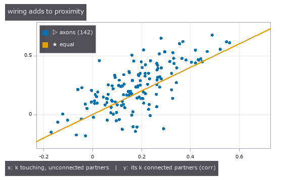
↑ each axon’s response predicted from the mean response of its connected partners (y) versus the same number of touching-but-unconnected partners (x): a…
↑ every number, with the bar it had to clear
↑ The animation ―― the measured responses of the 148 proofread axons (pale yellow) driven through the reservoir of the 4096-node connected subgraph over all somata (grey): a target lights when the drive it receives through its real synapses is in its own top quartile; correlation of the reservoir states with the measured responses 0.085 vs 0.048 for a degree-preserving shuffle
py -3.11 examples/poc_microns_brain_wave.py
Source: examples/poc_microns_brain_wave.py
This run produced 5 figures in total - see them all
Ops used (notes): graph_activity_spread · graph_degree_preserving_shuffle · graph_from_synapses · points_activity_video · reservoir_states
No.2026.132 —— Branch Territories — Handing Every Voxel Its Nearest Branch, Not Just Its Distance, Makes Per-Branch Volume and Radius Countable
A neuron cut out of serial EM sections becomes a graph of branches once skeletonised, but the per-branch volume and radius that morphometry needs (the compartment parameters of cable theory) can only be counted after every voxel of the volume is told which branch it belongs to. A distance transform returns how far the nearest skeleton is (a value) and discards which skeleton voxel is nearest (a direction), so on its own it cannot draw branch territories. On a synthetic dendrite with true branch labels (5 branches of different radius, one detached piece, 6 debris blobs), the pieces are held per component by vol_rle_components and selected by volume (8 components, 2 kept, 6 debris dropped), the branch ids of skeletonize_vol -> skeleton_branches3d are placed on the skeleton, and vol_nearest_label hands every voxel the id of its nearest branch (a Voronoi partition) which is then cut to the piece: the territories agree with the true nearest axis on 0.978 of the voxels and the per-branch volumes are within 2.9 %. The radius from vol_nearest_seed_vector (surface-to-skeleton displacement) plus 0.5 (the surface voxel centre sits half a voxel inside the boundary) is within 0.24 voxel for every branch, the same accuracy as the classic distance transform on the skeleton (0.23 voxel), but this one gives a radius at every surface voxel. The value-only classic (carve balls around the junctions, then connected components) either fails to separate the branches when the ball is small (agreement 0.63-0.65 for r = 0-4) or throws volume away when it is large (0.78 at r = 6 with 22 % unassigned) - the evidence that the direction is needed. Honest breakdown: skeleton branches end at every junction, so the trunk becomes three branch ids (9 ids onto 6 true branches, matched by majority overlap), and the +0.5 on the radius is a known discretisation bias added explicitly.
↑ Branch Territories — Handing Every Voxel Its Nearest Branch, Not Just Its Distance, Makes Per-Branch Volume and Radius Countable ―― A neuron cut out of serial EM sections becomes a graph of branches once skeletonised, but the per-branch volume and radius that morphometry needs (the compartment parameters of cable theory) can only be counted after every voxel of the volume is told which branch it belongs to. A distance transform returns how far the nearest skeleton is (a value) and discards which skeleton voxel is nearest (a direction), so on its own it cannot draw branch territories. On a synthetic dendrite with true branch labels (5 branches of different radius, one detached piece, 6 debris blobs), the pieces are held per component by vol_rle_components and selected by volume (8 components, 2 kept, 6 debris dropped), the branch ids of skeletonize_vol -> skeleton_branches3d are placed on the skeleton, and vol_nearest_label hands every voxel the id of its nearest branch (a Voronoi partition) which is then cut to the piece: the territories agree with the true nearest axis on 0.978 of the voxels and the per-branch volumes are within 2.9 %. The radius from vol_nearest_seed_vector (surface-to-skeleton displacement) plus 0.5 (the surface voxel centre sits half a voxel inside the boundary) is within 0.24 voxel for every branch, the same accuracy as the classic distance transform on the skeleton (0.23 voxel), but this one gives a radius at every surface voxel. The value-only classic (carve balls around the junctions, then connected components) either fails to separate the branches when the ball is small (agreement 0.63-0.65 for r = 0-4) or throws volume away when it is large (0.78 at r = 6 with 22 % unassigned) - the evidence that the direction is needed. Honest breakdown: skeleton branches end at every junction, so the trunk becomes three branch ids (9 ids onto 6 true branches, matched by majority overlap), and the +0.5 on the radius is a known discretisation bias added explicitly.
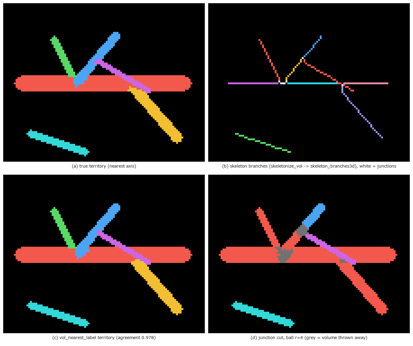
↑ The measurement ―― z projection of the synthetic dendrite: every voxel gets the branch whose skeleton is nearest, so the branch volumes can be counted; cutting balls around the junctions instead either fails to separate the branches or throws volume away (figure labels are in Japanese; the numbers are the same)

↑ both readings recover the radius of every branch to within half a voxel (the surface voxel centre sits half a voxel inside the boundary, hence the +0.…

↑ volume per branch comes from the territory; the junction-cut rows show that no ball radius separates the branches without throwing volume away
py -3.11 examples/poc_em_branch_territory.py
Source: examples/poc_em_branch_territory.py
This run produced 4 figures in total - see them all
Ops used (notes): identity · points_activity_video · skeleton · skeleton_branches3d · skeleton_graph3d · skeletonize_vol · vol_distance_transform · vol_label · vol_nearest_label · vol_nearest_seed_vector · vol_rle_components · vol_rle_decode · vol_rle_volume
No.2026.153 —— Is the Worm’s Wiring Bilaterally Symmetric? — The L/R-Swap Jaccard (set-overlap coefficient), Bracketed by a Closed Form and a Degree-Preserving Null
| The chemical-synapse wiring of the C. elegans hermaphrodite (Cook 2019; n=300, | E | =3,669, 98 left/right pairs): the edge-set overlap (Jaccard) between the wiring and the same wiring with every L/R pair swapped. The measured 0.473 sits between perfect symmetry (1.000) and a degree-preserving null that rewires edges while keeping every degree (0.080 ± 0.002, z 159). Ground truth is a counting closed form: in a mirrored synthetic wiring with m edges per side, moving k right-hand edges gives Jaccard = (m−k)/(m+k), and the op matches it down to the integer numerator and denominator at all 16 steps k=0..120. Per-pair asymmetry falls smoothly from 0.7 to 0.15 — the expected “concentration in a few pairs” turned out to be only about twice uniform (top 10 pairs carry 20 %, uniform would be 10 %). Leading pairs: HSN 60 %, PVN 57 %, RMG 53 %, URX 48 %. No data is bundled; without it the example runs on the synthetic mirrored wiring (Jaccard 0.500 = (120−40)/(120+40)). |
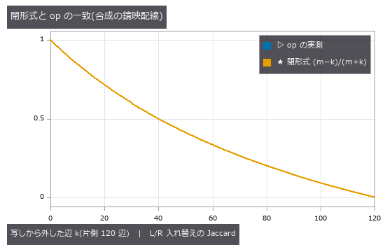
| *↑ Is the Worm’s Wiring Bilaterally Symmetric? — The L/R-Swap Jaccard (set-overlap coefficient), Bracketed by a Closed Form and a Degree-Preserving Null ―― The chemical-synapse wiring of the C. elegans hermaphrodite (Cook 2019; n=300, | E | =3,669, 98 left/right pairs): the edge-set overlap (Jaccard) between the wiring and the same wiring with every L/R pair swapped. The measured 0.473 sits between perfect symmetry (1.000) and a degree-preserving null that rewires edges while keeping every degree (0.080 ± 0.002, z 159). Ground truth is a counting closed form: in a mirrored synthetic wiring with m edges per side, moving k right-hand edges gives Jaccard = (m−k)/(m+k), and the op matches it down to the integer numerator and denominator at all 16 steps k=0..120. Per-pair asymmetry falls smoothly from 0.7 to 0.15 — the expected “concentration in a few pairs” turned out to be only about twice uniform (top 10 pairs carry 20 %, uniform would be 10 %). Leading pairs: HSN 60 %, PVN 57 %, RMG 53 %, URX 48 %. No data is bundled; without it the example runs on the synthetic mirrored wiring (Jaccard 0.500 = (120−40)/(120+40)).* |
Terms: Jaccard — A 0-to-1 set-similarity score equal to intersection size divided by union size.
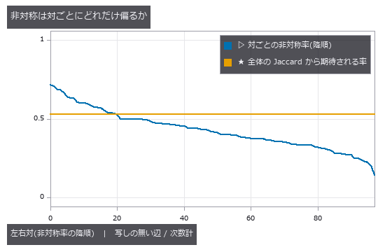
↑ The measurement ―― C. elegans 雌雄同体・化学シナプス(Cook 2019)。98 組のうち上位 10 組が非対称辺の 20 %(一様なら 10 %)。水平線は全体の Jaccard からの期待率 1 − J。 (figure labels are in Japanese; the numbers are the same)
py -3.11 examples/poc_connectome_lr_symmetry.py
Source: examples/poc_connectome_lr_symmetry.py
This run produced 2 figures in total - see them all
Ops used (notes): graph_degree_summary · graph_swap_symmetry
No.2026.156 —— How Much of the Wiring Do Two Genetically Identical Worms Share? — Counting the Connections Present in All 8 Worms of a Developmental Series
The chemical-synapse wiring of 8 genetically identical C. elegans (Witvliet 2021, from birth to adulthood), stacked on the 183 cells present in all 8, with graph_edge_consensus counting how many worms carry each connection. 442 connections are present in all 8 worms; a degree-preserving null that rewires every worm independently while keeping each cell’s in- and out-degree gives at most 0 in 20 samples. This core is 15 % of the 2,977 connections in the union but carries 57 % of the synapses summed over the 8 worms. Pairwise Jaccard falls with the difference in estimated age (0.51 on average for neighbouring stages, 0.33-0.34 between the newborn and the adults), and the two same-age adults overlap by only 0.53 - no more than neighbouring stages. Along the developmental order, 701 connections appear and stay to the end while 55 disappear. Ground truth is a closed form on a synthetic series: with a core of C connections in every worm and u unique connections per worm, h[K] = C, h[1] = K*u, every pairwise Jaccard is C/(C+2u), and stable/added/lost/flicker = C/u/u/(K-2)u, matched by the op down to the integer. Against the paper: it calls a connection stable when present in at least 7 datasets and reports about 43 % of adult connections as stable, while a naive cell-level count gives 34.5 %. Matching the authors’ per-connection classification table shows that the paper labels every cell-level connection of a left/right pair stable once the pooled pair connection is present in at least 7 worms (48.9 %); that rule alone reproduces 789 of the paper’s 792 stable connections (99.6 %), and removing variable and dynamic connections first gives 45.4 %. No data is bundled (the nemanode.org data carries no explicit licence); without it the example runs on a synthetic series.

↑ How Much of the Wiring Do Two Genetically Identical Worms Share? — Counting the Connections Present in All 8 Worms of a Developmental Series ―― The chemical-synapse wiring of 8 genetically identical C. elegans (Witvliet 2021, from birth to adulthood), stacked on the 183 cells present in all 8, with graph_edge_consensus counting how many worms carry each connection. 442 connections are present in all 8 worms; a degree-preserving null that rewires every worm independently while keeping each cell’s in- and out-degree gives at most 0 in 20 samples. This core is 15 % of the 2,977 connections in the union but carries 57 % of the synapses summed over the 8 worms. Pairwise Jaccard falls with the difference in estimated age (0.51 on average for neighbouring stages, 0.33-0.34 between the newborn and the adults), and the two same-age adults overlap by only 0.53 - no more than neighbouring stages. Along the developmental order, 701 connections appear and stay to the end while 55 disappear. Ground truth is a closed form on a synthetic series: with a core of C connections in every worm and u unique connections per worm, h[K] = C, h[1] = Ku, every pairwise Jaccard is C/(C+2u), and stable/added/lost/flicker = C/u/u/(K-2)u, matched by the op down to the integer. Against the paper: it calls a connection stable when present in at least 7 datasets and reports about 43 % of adult connections as stable, while a naive cell-level count gives 34.5 %. Matching the authors’ per-connection classification table shows that the paper labels every cell-level connection of a left/right pair stable once the pooled pair connection is present in at least 7 worms (48.9 %); that rule alone reproduces 789 of the paper’s 792 stable connections (99.6 %), and removing variable and dynamic connections first gives 45.4 %. No data is bundled (the nemanode.org data carries no explicit licence); without it the example runs on a synthetic series.*
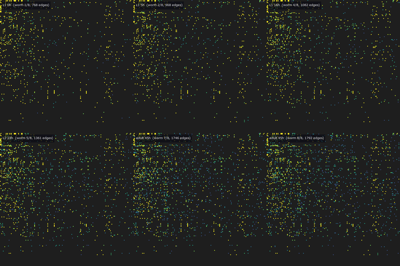
↑ The measurement ―― 生まれた直後から成虫まで 8 匹の配線を順に。色は全体での出現回数なので、早い段階から在る結合ほど明るい。 (figure labels are in Japanese; the numbers are the same)
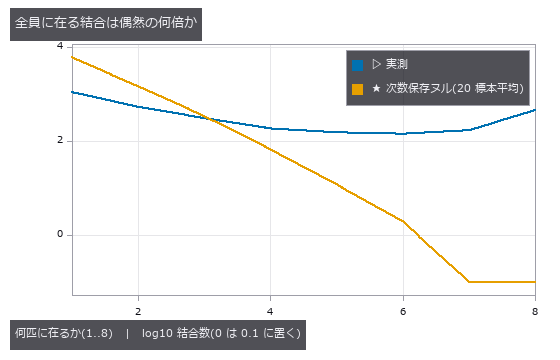
↑ ヌルは各個体の入次数・出次数を保ったまま独立に組み替えた配線。
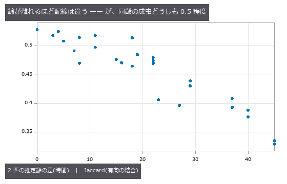
↑ 横軸 0 の点が同齢の成虫 2 匹(Jaccard 0.53)。
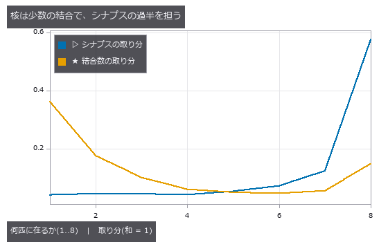
↑ 8 匹全員に在る結合は結合数の 15 %、シナプスの 57 %。
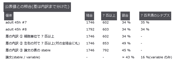
↑ 論文は左右の対でまとめた結合が 7 匹以上に在れば、その対の細胞単位の結合すべてに stable の札を付ける(②)。
py -3.11 examples/poc_connectome_across_worms.py
Source: examples/poc_connectome_across_worms.py
This run produced 6 figures in total - see them all
Ops used (notes): graph_edge_consensus · intersection · text_box
No.2026.157 —— How Much Does a Hand-Traced Wiring Diagram from 40 Years Ago Overlap Today’s Adult Worms? — The Era Difference Next to the Individual Difference
The origin of C. elegans wiring diagrams, White 1986 (hand-traced from electron micrographs, adult N2U), stacked with the two adults of Witvliet 2021 on their 215 common cells with graph_edge_consensus. The overlap (Jaccard) is 0.508 between the two adults reconstructed the same way and 0.431 / 0.442 between 1986 N2U and the 2021 adults: the era-and-method difference is 0.07, small next to the individual difference 1 - 0.508 = 0.49. 1,015 connections are present in all three, 36 times the 28 of a degree-preserving null. The 451 connections present in both 2021 adults but missing in 1986 are thin (2.0 synapses on average), clearly separated from those present in all three (5.7). Found by the checks: binning the rounded mean of two animals produced an odd/even zigzag from numpy’s round-half-to-even (2.5 -> 2); counting the integer sum removed it. Honest breakdown: the N2U on nemanode was supplemented with muscles by the Zhen lab in 2020, so the era difference includes re-annotation; JSH is an L4 larva and is left out. No data is bundled; without it the example runs on a synthetic set.

↑ How Much Does a Hand-Traced Wiring Diagram from 40 Years Ago Overlap Today’s Adult Worms? — The Era Difference Next to the Individual Difference ―― The origin of C. elegans wiring diagrams, White 1986 (hand-traced from electron micrographs, adult N2U), stacked with the two adults of Witvliet 2021 on their 215 common cells with graph_edge_consensus. The overlap (Jaccard) is 0.508 between the two adults reconstructed the same way and 0.431 / 0.442 between 1986 N2U and the 2021 adults: the era-and-method difference is 0.07, small next to the individual difference 1 - 0.508 = 0.49. 1,015 connections are present in all three, 36 times the 28 of a degree-preserving null. The 451 connections present in both 2021 adults but missing in 1986 are thin (2.0 synapses on average), clearly separated from those present in all three (5.7). Found by the checks: binning the rounded mean of two animals produced an odd/even zigzag from numpy’s round-half-to-even (2.5 -> 2); counting the integer sum removed it. Honest breakdown: the N2U on nemanode was supplemented with muscles by the Zhen lab in 2020, so the era difference includes re-annotation; JSH is an L4 larva and is left out. No data is bundled; without it the example runs on a synthetic set.
Terms: Jaccard — A 0-to-1 set-similarity score equal to intersection size divided by union size.

↑ The measurement ―― 3 匹すべてに在る結合 1015 本、ヌルの平均 28.2 本。 (figure labels are in Japanese; the numbers are the same)
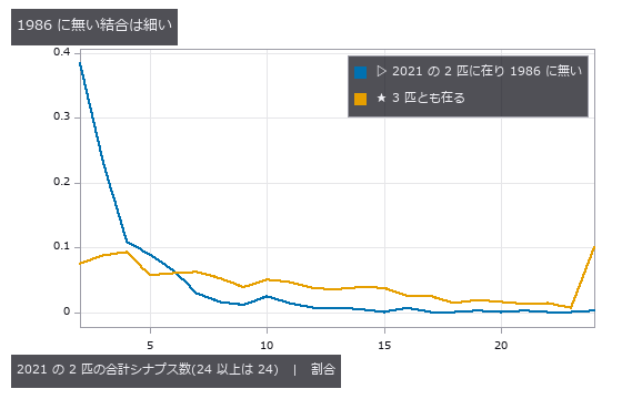
↑ 2021 の 2 匹ともに在るのに 1986 に無い結合は平均 2.01 シナプス、3 匹とも在る結合は 5.73。
py -3.11 examples/poc_connectome_across_decades.py
Source: examples/poc_connectome_across_decades.py
This run produced 3 figures in total - see them all
Ops used (notes): graph_edge_consensus · intersection
No.2026.158 —— How Much Do a Worm’s Neurites Grow from Birth to Adulthood? — Measuring Eight Animals’ Skeletons with the Tree Ops and Setting the Result Beside the Paper
| The neurite skeletons of the 8 C. elegans of Witvliet 2021 (birth to adult), converted to SWC trees and measured with tree_from_swc / tree_morphometry / tree_sholl. 1,727 trees (the 61 skeletons that break into fragments are measured per fragment and summed) all pass the structural promises (one root, parent id < child id, nodes = edges + 1) and the Sholl closed form (area under the curve = sum | d_child - d_parent | ). Second implementation: on the 1,586 single-fragment skeletons the op’s longest path matches the maximum of the authors’ per-node dist_to_root to a relative 1.75e-9. Found by the checks: the authors’ length field is not the sum of segment lengths (median 0.89 of it; 1,360 of 1,586 disagree) and cannot be a gate; dist_to_root also lists nodes without coordinates (54 of 196 skeletons in the first animal), so only nodes with coordinates are compared; writing coordinates to SWC with 3 decimals shifted the path by 1.9e-6. Total length grows from 2,806 um at birth to 12,038 um in the adult, 4.29-fold (3.86-fold on the 195 cells present in all 8), against about 5-fold in the paper; summing the authors’ own length field also gives 3.95-fold, so the 5-fold itself does not come out of a plain sum of this file (the order of magnitude agrees). The L3 total is close to L2 because of specimen shrinkage, which the authors correct by 1.1. No data is bundled. |
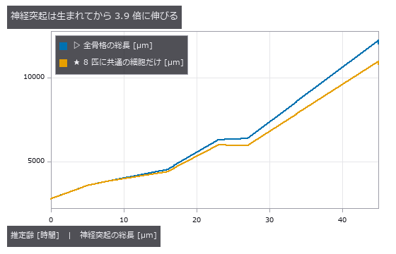
| *↑ How Much Do a Worm’s Neurites Grow from Birth to Adulthood? — Measuring Eight Animals’ Skeletons with the Tree Ops and Setting the Result Beside the Paper ―― The neurite skeletons of the 8 C. elegans of Witvliet 2021 (birth to adult), converted to SWC trees and measured with tree_from_swc / tree_morphometry / tree_sholl. 1,727 trees (the 61 skeletons that break into fragments are measured per fragment and summed) all pass the structural promises (one root, parent id < child id, nodes = edges + 1) and the Sholl closed form (area under the curve = sum | d_child - d_parent | ). Second implementation: on the 1,586 single-fragment skeletons the op’s longest path matches the maximum of the authors’ per-node dist_to_root to a relative 1.75e-9. Found by the checks: the authors’ length field is not the sum of segment lengths (median 0.89 of it; 1,360 of 1,586 disagree) and cannot be a gate; dist_to_root also lists nodes without coordinates (54 of 196 skeletons in the first animal), so only nodes with coordinates are compared; writing coordinates to SWC with 3 decimals shifted the path by 1.9e-6. Total length grows from 2,806 um at birth to 12,038 um in the adult, 4.29-fold (3.86-fold on the 195 cells present in all 8), against about 5-fold in the paper; summing the authors’ own length field also gives 3.95-fold, so the 5-fold itself does not come out of a plain sum of this file (the order of magnitude agrees). The L3 total is close to L2 because of specimen shrinkage, which the authors correct by 1.1. No data is bundled.* |
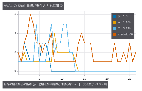
↑ The measurement ―― 同じ名前のニューロン AVAL を 4 つの発生段階で。3-D の Sholl なので回転に依らない。 (figure labels are in Japanese; the numbers are the same)
py -3.11 examples/poc_worm_neurites_grow.py
Source: examples/poc_worm_neurites_grow.py
This run produced 2 figures in total - see them all
Ops used (notes): intersection · tree_from_swc · tree_morphometry · tree_sholl
No.2026.159 —— Scoring Neuron Segmentations from Electron Microscopy — Over-Splitting and Over-Merging as Two Separate Numbers
The errors of automatic neuron segmentation for connectomics are of two kinds: a split cuts one neuron into two, a merge glues two neurons into one. seg_variation_of_information returns VOI divided into split and merge. Injecting one error at a time into the ground truth of CREMI sample A (z = 40, 512 squared) with the existing seg_inject_split / seg_inject_merge, the 4 splits raise only split and the 4 merges only merge, each by exactly (m/N)·H2(m1/m) bits (error < 1e-12; exact for any division of real data). A classic segmentation (membrane response -> threshold -> connected components -> membrane pixels assigned to the nearest cell) goes from over-split at the 60th percentile (split 1.14 / merge 0.18) to over-merged at the 85th (split 0.05 / merge 5.02), with the lowest VOI (1.263) at the 65th, just before the crossing. Found by the checks: leaving membrane pixels as background (label 0) counts the whole background as one huge region and inflates merge 2.4-fold (2.07 against 0.85 at the 70th percentile), making every threshold look over-merged. scikit-image, the second implementation, agrees on the adapted Rand error, but its precision is divided by the truth pairs, the opposite of its docstring. Raw data is not bundled.
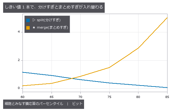
↑ Scoring Neuron Segmentations from Electron Microscopy — Over-Splitting and Over-Merging as Two Separate Numbers ―― The errors of automatic neuron segmentation for connectomics are of two kinds: a split cuts one neuron into two, a merge glues two neurons into one. seg_variation_of_information returns VOI divided into split and merge. Injecting one error at a time into the ground truth of CREMI sample A (z = 40, 512 squared) with the existing seg_inject_split / seg_inject_merge, the 4 splits raise only split and the 4 merges only merge, each by exactly (m/N)·H2(m1/m) bits (error < 1e-12; exact for any division of real data). A classic segmentation (membrane response -> threshold -> connected components -> membrane pixels assigned to the nearest cell) goes from over-split at the 60th percentile (split 1.14 / merge 0.18) to over-merged at the 85th (split 0.05 / merge 5.02), with the lowest VOI (1.263) at the 65th, just before the crossing. Found by the checks: leaving membrane pixels as background (label 0) counts the whole background as one huge region and inflates merge 2.4-fold (2.07 against 0.85 at the 70th percentile), making every threshold look over-merged. scikit-image, the second implementation, agrees on the adapted Rand error, but its precision is divided by the truth pairs, the opposite of its docstring. Raw data is not bundled.
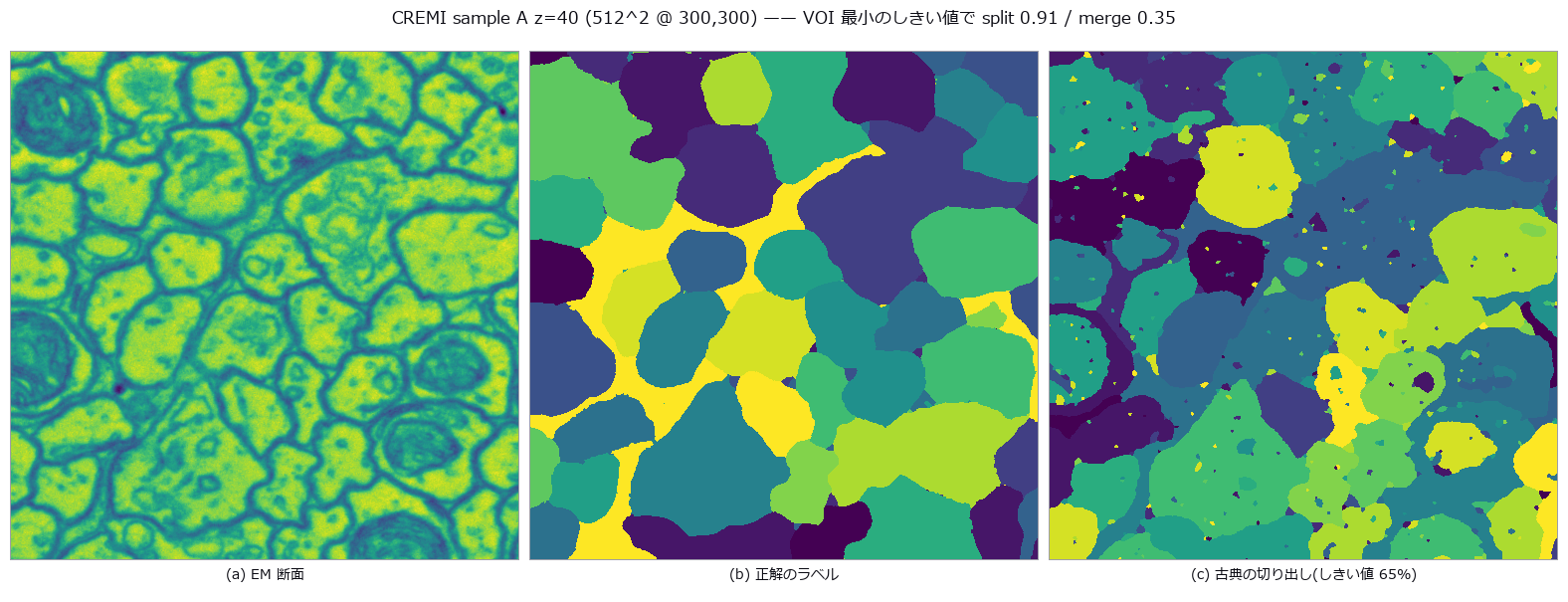
↑ The measurement (figure labels are in Japanese; the numbers are the same)
py -3.11 examples/poc_em_split_merge_score.py
Source: examples/poc_em_split_merge_score.py
This run produced 2 figures in total - see them all
Ops used (notes): blob_label · seg_inject_merge · seg_inject_split · seg_label_changes · seg_membrane_response · seg_rand · seg_variation_of_information
No.2026.160 —— Where Segmentation Errors Break the Wiring Diagram — Pixel Scores Overweight Splits and Underweight Merges
A connectome is read by dropping synapse annotations (a pre and a post point) onto segmented neurons, so segmentation errors turn into wiring errors — but not all of them. seg_wiring_variation retakes the pixel VOI at the 2n synapse ends only. This construction is the synapse VI of Plaza et al. 2014 (Focused proofreading); what is new here is the numpy-only implementation, the connection level, the injection experiment and the proofreading-order comparison. On the ground truth of CREMI sample A (125 slices × 625 squared, 115 synapses, 107 connections), one error at a time was injected into each of the 54 neurons carrying synapses: cut in half at the median x, or glued to the neighbour it touches most. The ends VOI matched the closed form (s/2n)·H2(s1/s) in all 108 cases (largest error 1.4e-17). 23 of the 54 cuts change the wiring by not a single bit (no synapse end on one side of the cut). Wiring damage per pixel bit (median) is 1.30 for merges and 0.58 for splits; the rank correlation of pixel and ends VOI is 0.60. Fixing the top 20 errors by pixel VOI removes 41 % of the wiring damage — far better than random (19 %) but short of the wiring order (49 %). Found by the checks: computing a conditional entropy as H(a,b) − H(a) left 8.9e-16 of rounding dust on a pure relabelling and failed the ‘identical means 0’ gate; the direct sum −Σ p log2(n_ij / n_i) makes it exactly 0. VOI over synapses grouped by connection alone stays 0 when a one-synapse connection is cut (most of the 107), so the ends level is primary. The same errors are also scored by NRI (Reilly 2018, the F-score of pairs of ends; the new op seg_synapse_nri, exactly 1 − adapted Rand error over the ends), with the gate that an error costing 0 ends-VOI bits also costs 0 NRI. The rank correlation of NRI loss with ends VOI is 1.00, with pixel VOI 0.59. Inside 1.30 / 0.58: each error’s wiring / pixel ratio is identically density × balance (a gate on all 108). Merges have balance ≈ 1 so their ratio is the density; the cut discount comes mostly from how few ends a neuron has (median 3: even evenly spread ends give an expected H2 of 0.62 by the binomial closed form, measured 0.53). The new op seg_wiring_exposure returns the count-only prediction per neuron (bound s/2n, binomial expectation); over the 54 cuts 0.677 measured / 0.788 predicted / 1.000 bound. Raw data is not bundled.
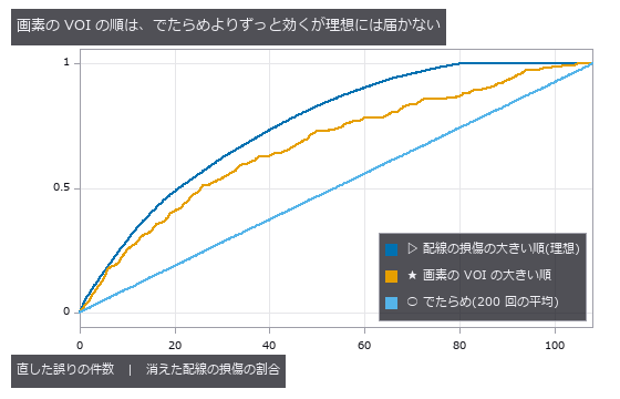
↑ Where Segmentation Errors Break the Wiring Diagram — Pixel Scores Overweight Splits and Underweight Merges ―― A connectome is read by dropping synapse annotations (a pre and a post point) onto segmented neurons, so segmentation errors turn into wiring errors — but not all of them. seg_wiring_variation retakes the pixel VOI at the 2n synapse ends only. This construction is the synapse VI of Plaza et al. 2014 (Focused proofreading); what is new here is the numpy-only implementation, the connection level, the injection experiment and the proofreading-order comparison. On the ground truth of CREMI sample A (125 slices × 625 squared, 115 synapses, 107 connections), one error at a time was injected into each of the 54 neurons carrying synapses: cut in half at the median x, or glued to the neighbour it touches most. The ends VOI matched the closed form (s/2n)·H2(s1/s) in all 108 cases (largest error 1.4e-17). 23 of the 54 cuts change the wiring by not a single bit (no synapse end on one side of the cut). Wiring damage per pixel bit (median) is 1.30 for merges and 0.58 for splits; the rank correlation of pixel and ends VOI is 0.60. Fixing the top 20 errors by pixel VOI removes 41 % of the wiring damage — far better than random (19 %) but short of the wiring order (49 %). Found by the checks: computing a conditional entropy as H(a,b) − H(a) left 8.9e-16 of rounding dust on a pure relabelling and failed the ‘identical means 0’ gate; the direct sum −Σ p log2(n_ij / n_i) makes it exactly 0. VOI over synapses grouped by connection alone stays 0 when a one-synapse connection is cut (most of the 107), so the ends level is primary. The same errors are also scored by NRI (Reilly 2018, the F-score of pairs of ends; the new op seg_synapse_nri, exactly 1 − adapted Rand error over the ends), with the gate that an error costing 0 ends-VOI bits also costs 0 NRI. The rank correlation of NRI loss with ends VOI is 1.00, with pixel VOI 0.59. Inside 1.30 / 0.58: each error’s wiring / pixel ratio is identically density × balance (a gate on all 108). Merges have balance ≈ 1 so their ratio is the density; the cut discount comes mostly from how few ends a neuron has (median 3: even evenly spread ends give an expected H2 of 0.62 by the binomial closed form, measured 0.53). The new op seg_wiring_exposure returns the count-only prediction per neuron (bound s/2n, binomial expectation); over the 54 cuts 0.677 measured / 0.788 predicted / 1.000 bound. Raw data is not bundled.
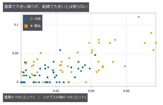
↑ The measurement ―― 1 点 = 仕込んだ誤り 1 件。順位相関 0.60。分断の 23 / 54 件は配線を 1 ビットも変えない(横軸の上に並ぶ)。 (figure labels are in Japanese; the numbers are the same)
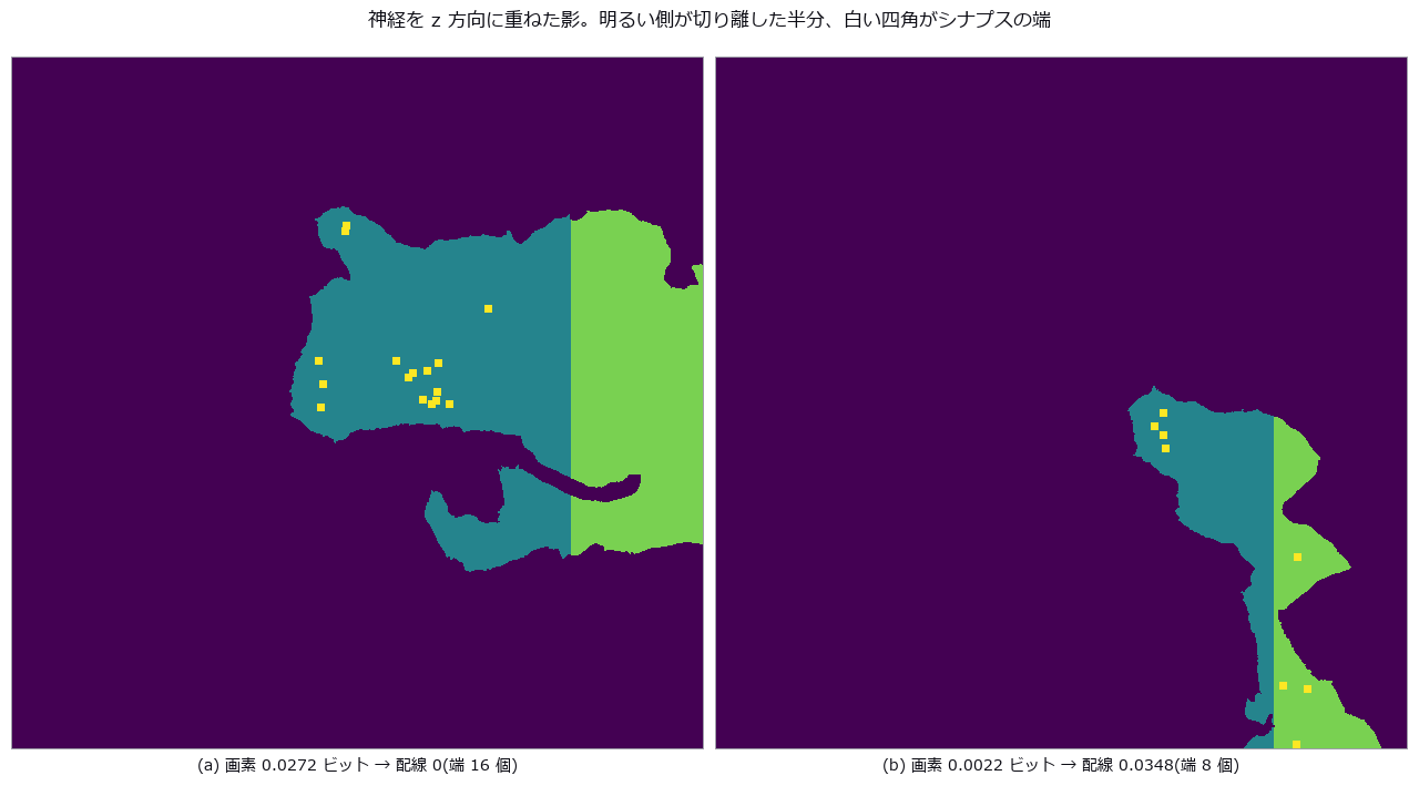
↑ この回の図
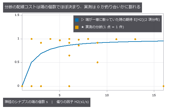
↑ CREMI sample A(z 125 枚 × xy 625² @ 0,625)。
py -3.11 examples/poc_em_wiring_errors.py
Source: examples/poc_em_wiring_errors.py
This run produced 4 figures in total - see them all
Ops used (notes): seg_synapse_nri · seg_synapse_partners · seg_variation_of_information · seg_wiring_exposure · seg_wiring_variation
No.2026.161 —— Do Synapses Grow in Proportion to Neurites? — Shape Growth and Wiring Growth Set Side by Side, Cell by Cell, in Eight Worms
Witvliet 2021’s eight animals carry both a skeleton (shape) and a wiring diagram (synapses) per individual. From the total neurite length measured by the tree ops and the total number of chemical synapses, density rises ×1.32 from 0.462 /µm at birth to 0.611 at 16 h of L1, and afterwards wobbles (max / min) by 1.14 — consistent with the paper’s “density is maintained except during L1” (the gate is “the L1 rise exceeds the later wobble”, with no number hard-coded). Cell by cell, over the 178 cells with a skeleton and synapses in both animals 1 and 8, the rank correlation between neurite growth (median ×3.7) and synapse gain (median ×6.0) is 0.23 (97.5th percentile of a cell-shuffling null: 0.17): not zero, but shape alone does not decide it. Density rose in 82 % of cells. Comparing the matrices of animals 1 and 8 with the new op graph_strength_growth, of the 6,674 new synapses 3,232 thickened existing connections, 3,627 made new ones, −159 were on connections that vanished and −26 on ones that thinned (the four sum exactly to 6,674). The rank correlation between partners at birth and the gain is 0.58 for inputs / 0.51 for outputs, and the top-decile hubs’ share falls from 34 % to 28 % of inputs and 24 % to 20 % of outputs — “hubs disproportionately add inputs” does not appear under this definition (the paper’s quantity is defined differently, so this is not a contradiction). Raw data is not bundled.
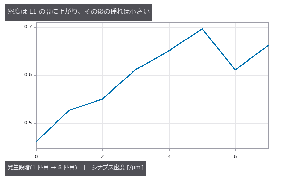
↑ Do Synapses Grow in Proportion to Neurites? — Shape Growth and Wiring Growth Set Side by Side, Cell by Cell, in Eight Worms ―― Witvliet 2021’s eight animals carry both a skeleton (shape) and a wiring diagram (synapses) per individual. From the total neurite length measured by the tree ops and the total number of chemical synapses, density rises ×1.32 from 0.462 /µm at birth to 0.611 at 16 h of L1, and afterwards wobbles (max / min) by 1.14 — consistent with the paper’s “density is maintained except during L1” (the gate is “the L1 rise exceeds the later wobble”, with no number hard-coded). Cell by cell, over the 178 cells with a skeleton and synapses in both animals 1 and 8, the rank correlation between neurite growth (median ×3.7) and synapse gain (median ×6.0) is 0.23 (97.5th percentile of a cell-shuffling null: 0.17): not zero, but shape alone does not decide it. Density rose in 82 % of cells. Comparing the matrices of animals 1 and 8 with the new op graph_strength_growth, of the 6,674 new synapses 3,232 thickened existing connections, 3,627 made new ones, −159 were on connections that vanished and −26 on ones that thinned (the four sum exactly to 6,674). The rank correlation between partners at birth and the gain is 0.58 for inputs / 0.51 for outputs, and the top-decile hubs’ share falls from 34 % to 28 % of inputs and 24 % to 20 % of outputs — “hubs disproportionately add inputs” does not appear under this definition (the paper’s quantity is defined differently, so this is not a contradiction). Raw data is not bundled.
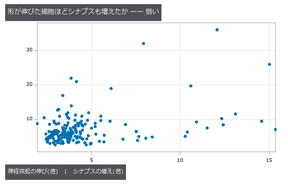
↑ The measurement ―― 1 点 = 細胞 178 個。順位相関 0.23(零分布 97.5 % 点 0.17)。 (figure labels are in Japanese; the numbers are the same)
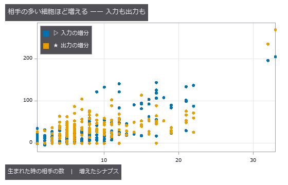
↑ 順位相関 入力 0.58 / 出力 0.51。
py -3.11 examples/poc_worm_synapses_vs_neurites.py
Source: examples/poc_worm_synapses_vs_neurites.py
This run produced 3 figures in total - see them all
Ops used (notes): graph_strength_growth · tree_from_swc · tree_morphometry
No.2026.162 —— Run Length Forgives No Small Merge — ERL and VOI Weigh the Same Error Differently
| Automatic segmentations are scored either by VOI (split / merge, from the contingency table) or by ERL (expected run length, Januszewski 2018): how far along the ground-truth skeleton one can travel inside one object. The new op tree_run_length counts the runs of a skeleton painted with candidate labels and treats runs of merged objects as length 0. With Witvliet 2021’s 1,713 skeletons (12+ nodes) as ground truth, one candidate error at a time was injected (the candidates are synthetic, not a segmenter’s output). One cut: ERL matches the closed form (A² + (L − A − | e | )²)/L (A = cable of the cut-off subtree, counted by a second traversal) on all 1,713 skeletons (relative 4e-15), and VOI split matches (m/N)·H2 (3.5e-16). On 100 unbranched skeletons, cutting in the middle leaves ERL at 0.48 L, cutting near an end 0.80 L. Gluing the far q of skeleton a onto skeleton b’s object (856 pairs): VOI merge rises monotonically from 0.142 bits at q = 5 % to 0.662 at 50 %, while the ERL of the receiving skeleton b is 0 for every q (loss 1.000) and a’s loss follows the cut formula 1 − (1 − q)². Cutting 65 unbranched skeletons at 3 points uniform along the cable, the run fractions follow Dirichlet(1,…,1): mean Σl²/L’² ÷ 2/(m+2) = 1.023. Found by the checks: the first version claimed that a’s loss was independent of q — wrong; ERL zeroes the runs of the merged object, and the rest of a survives intact; the constant loss falls on b, which that object covers entirely. Sampling cut positions uniformly over node indices instead of cable biased the ratio to 0.945, because edge lengths are uneven. Raw data is not bundled. |
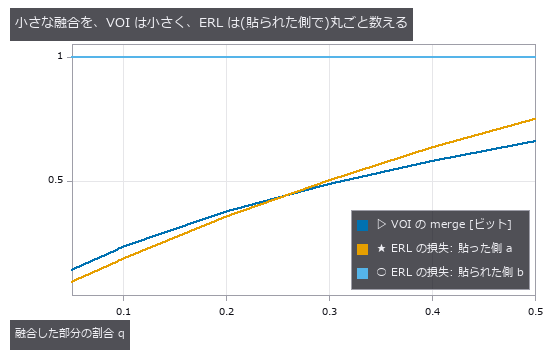
| *↑ Run Length Forgives No Small Merge — ERL and VOI Weigh the Same Error Differently ―― Automatic segmentations are scored either by VOI (split / merge, from the contingency table) or by ERL (expected run length, Januszewski 2018): how far along the ground-truth skeleton one can travel inside one object. The new op tree_run_length counts the runs of a skeleton painted with candidate labels and treats runs of merged objects as length 0. With Witvliet 2021’s 1,713 skeletons (12+ nodes) as ground truth, one candidate error at a time was injected (the candidates are synthetic, not a segmenter’s output). One cut: ERL matches the closed form (A² + (L − A − | e | )²)/L (A = cable of the cut-off subtree, counted by a second traversal) on all 1,713 skeletons (relative 4e-15), and VOI split matches (m/N)·H2 (3.5e-16). On 100 unbranched skeletons, cutting in the middle leaves ERL at 0.48 L, cutting near an end 0.80 L. Gluing the far q of skeleton a onto skeleton b’s object (856 pairs): VOI merge rises monotonically from 0.142 bits at q = 5 % to 0.662 at 50 %, while the ERL of the receiving skeleton b is 0 for every q (loss 1.000) and a’s loss follows the cut formula 1 − (1 − q)². Cutting 65 unbranched skeletons at 3 points uniform along the cable, the run fractions follow Dirichlet(1,…,1): mean Σl²/L’² ÷ 2/(m+2) = 1.023. Found by the checks: the first version claimed that a’s loss was independent of q — wrong; ERL zeroes the runs of the merged object, and the rest of a survives intact; the constant loss falls on b, which that object covers entirely. Sampling cut positions uniformly over node indices instead of cable biased the ratio to 0.945, because edge lengths are uneven. Raw data is not bundled.* |
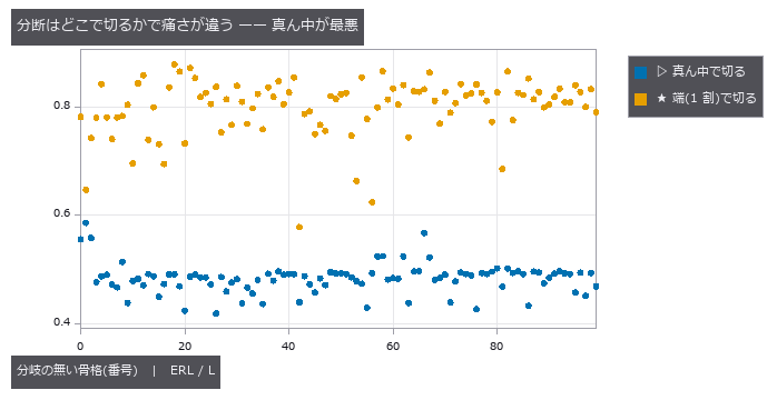
↑ The measurement ―― 1 点 = 骨格 1 本。真ん中で切ると ERL は L の約 1/2、端で切ると約 0.8 L。 (figure labels are in Japanese; the numbers are the same)
py -3.11 examples/poc_skeleton_run_length_vs_voi.py
Source: examples/poc_skeleton_run_length_vs_voi.py
This run produced 2 figures in total - see them all
Ops used (notes): seg_variation_of_information · tree_from_swc · tree_run_length
No.2026.163 —— Slime-Mould Tubes Solve the Maze — Thickening and Thinning Alone Converge to the Shortest Path, Bracketed by a Theorem and Dijkstra
| The slime mould Physarum leaves the shortest path of a maze by nothing more than thickening and thinning its tubes with the flow through them (Tero 2010). Its dynamics (Kirchhoff pressures, dD/dt = | Q | − D) are proved to converge to the indicator of the shortest path when it is unique (Bonifaci 2012). Two new ops run it — graph_physarum_path on a weighted graph and physarum_route on a cost image (neighbouring pixels joined by a tube of length (c_u+c_v)/2) — with Dijkstra (scipy) and route_through_array (skimage) as the truth. On five 15×15 lattices, a 21×21 perfect maze and a 32×32 terrain the mould’s route equals the minimum-cost path in every case (difference < 1e-9). At 600 iterations the lattice routes already match 5/5 (the Afterman PoC had 4/5); by 3,000 iterations 3/5 have converged to the indicator (> 0.99 on the path, < 0.01 elsewhere) and the two cut off are those whose gap to the runner-up route (the exact second-shortest, from Dijkstra with each edge of the shortest path removed in turn) is smallest, 0.009 and 0.032 — the gap sets the speed. The Lyapunov function V = Σ L·D fell in the maze from 227,280 to 133.60 (shortest path 133.59) without rising once over 23 intervals, and the inequality flow length Σ | Q | L ≥ shortest path held exactly throughout. Where many routes tie (uniform cost) the tubes never settle on one, and the op refuses. |
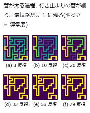
| *↑ Slime-Mould Tubes Solve the Maze — Thickening and Thinning Alone Converge to the Shortest Path, Bracketed by a Theorem and Dijkstra ―― The slime mould Physarum leaves the shortest path of a maze by nothing more than thickening and thinning its tubes with the flow through them (Tero 2010). Its dynamics (Kirchhoff pressures, dD/dt = | Q | − D) are proved to converge to the indicator of the shortest path when it is unique (Bonifaci 2012). Two new ops run it — graph_physarum_path on a weighted graph and physarum_route on a cost image (neighbouring pixels joined by a tube of length (c_u+c_v)/2) — with Dijkstra (scipy) and route_through_array (skimage) as the truth. On five 15×15 lattices, a 21×21 perfect maze and a 32×32 terrain the mould’s route equals the minimum-cost path in every case (difference < 1e-9). At 600 iterations the lattice routes already match 5/5 (the Afterman PoC had 4/5); by 3,000 iterations 3/5 have converged to the indicator (> 0.99 on the path, < 0.01 elsewhere) and the two cut off are those whose gap to the runner-up route (the exact second-shortest, from Dijkstra with each edge of the shortest path removed in turn) is smallest, 0.009 and 0.032 — the gap sets the speed. The Lyapunov function V = Σ L·D fell in the maze from 227,280 to 133.60 (shortest path 133.59) without rising once over 23 intervals, and the inequality flow length Σ | Q | L ≥ shortest path held exactly throughout. Where many routes tie (uniform cost) the tubes never settle on one, and the op refuses.* |

↑ The measurement ―― 同じ迷路、24 コマ。行き止まりから順に細り、最後に最短路だけが残る。 (figure labels are in Japanese; the numbers are the same)
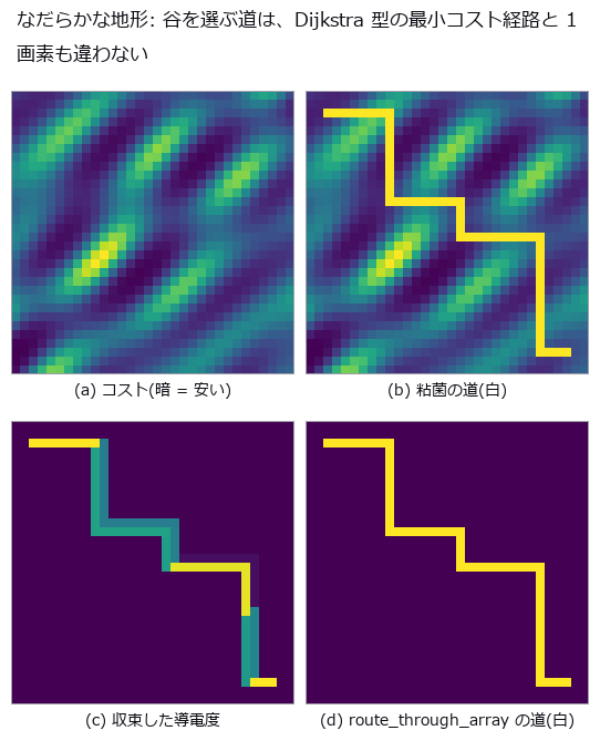
↑ 32×32。
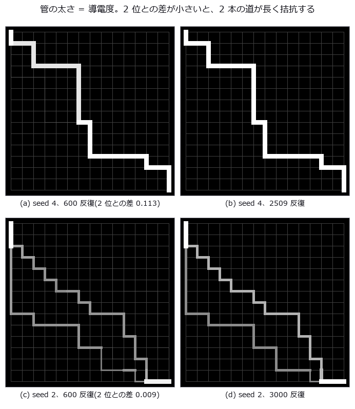
↑ 15×15 の格子、辺長 U(0.5, 1.5)、左上 → 右下。
py -3.11 examples/poc_physarum_maze.py
Source: examples/poc_physarum_maze.py
This run produced 4 figures in total - see them all
Ops used (notes): graph_physarum_path · physarum_route
No.2026.165 —— Slime Mould Solves Optimal Transport — Make the Source and Sink Mass Distributions and the Same Tube Dynamics Converge to the Earth Mover’s Distance
| The maze PoC had one source and one sink. Give the same dynamics (Kirchhoff pressures, Q = D (p_u − p_v)/L, dD/dt = | Q | − D) a supply vector (sum 0) instead, and it converges to L1 optimal transport on the graph — the Beckmann problem, i.e. the 1-Wasserstein distance (Bonifaci 2017; Facca, Karrenbauer, Kolev and Mehlhorn 2020; Facca, Cardin and Putti 2018 for the continuum). Two new ops, graph_physarum_transport (weighted graph + supply) and physarum_transport_image (two mass images, pixels joined by unit tubes = EMD in the Manhattan metric), return the cost Σ L | Q | (an upper bound) together with the Kantorovich–Rubinstein lower bound — b·φ for the McShane envelope φ of the pressure, made 1-Lipschitz. The true distance always lies between them, so the gap certifies how far the current flow is from optimal, and the run stops when it closes. Ten truths: on five random trees the closed form Σ L_e | subtree supply | matches to 1.7e-15 (the flow on a tree is unique; 37–38 iterations); on an uneven 1-D grid the existing op wasserstein_1d agrees at 0.316477; on a 12-vs-12 complete bipartite graph the Hungarian minimum assignment 0.163242 is met at 0.163244 (459 iterations) and the surviving tubes are exactly the optimal assignment (≥ 1.00 on it, ≤ 0.001 elsewhere); on a 6×6 grid of random mass the LP (HiGHS) optimum 0.591849 is matched; a disk shifted by (5, 8) pixels gives EMD 13.000086 = | dr | + | dc | as the theorem says; with one source and one sink the lower bound equals Dijkstra’s distance 9.367260049 exactly (the envelope of the pressure is the shortest-path potential). The metric axioms (symmetry, linearity in length and mass, triangle inequality) hold. Disk → two disks (24×24) reaches EMD 12.0001 in 183 iterations, filmed in 36 frames as the tubes form. 9.1 s in all. Honestly: the mould is not faster than the Hungarian algorithm or the network simplex. Its merits are that a local rule alone reaches the optimum, that it batches in parallel, and that it certifies its own answer. |

| *↑ Slime Mould Solves Optimal Transport — Make the Source and Sink Mass Distributions and the Same Tube Dynamics Converge to the Earth Mover’s Distance ―― The maze PoC had one source and one sink. Give the same dynamics (Kirchhoff pressures, Q = D (p_u − p_v)/L, dD/dt = | Q | − D) a supply vector (sum 0) instead, and it converges to L1 optimal transport on the graph — the Beckmann problem, i.e. the 1-Wasserstein distance (Bonifaci 2017; Facca, Karrenbauer, Kolev and Mehlhorn 2020; Facca, Cardin and Putti 2018 for the continuum). Two new ops, graph_physarum_transport (weighted graph + supply) and physarum_transport_image (two mass images, pixels joined by unit tubes = EMD in the Manhattan metric), return the cost Σ L | Q | (an upper bound) together with the Kantorovich–Rubinstein lower bound — b·φ for the McShane envelope φ of the pressure, made 1-Lipschitz. The true distance always lies between them, so the gap certifies how far the current flow is from optimal, and the run stops when it closes. Ten truths: on five random trees the closed form Σ L_e | subtree supply | matches to 1.7e-15 (the flow on a tree is unique; 37–38 iterations); on an uneven 1-D grid the existing op wasserstein_1d agrees at 0.316477; on a 12-vs-12 complete bipartite graph the Hungarian minimum assignment 0.163242 is met at 0.163244 (459 iterations) and the surviving tubes are exactly the optimal assignment (≥ 1.00 on it, ≤ 0.001 elsewhere); on a 6×6 grid of random mass the LP (HiGHS) optimum 0.591849 is matched; a disk shifted by (5, 8) pixels gives EMD 13.000086 = | dr | + | dc | as the theorem says; with one source and one sink the lower bound equals Dijkstra’s distance 9.367260049 exactly (the envelope of the pressure is the shortest-path potential). The metric axioms (symmetry, linearity in length and mass, triangle inequality) hold. Disk → two disks (24×24) reaches EMD 12.0001 in 183 iterations, filmed in 36 frames as the tubes form. 9.1 s in all. Honestly: the mould is not faster than the Hungarian algorithm or the network simplex. Its merits are that a local rule alone reaches the optimum, that it batches in parallel, and that it certifies its own answer.* |

↑ The measurement ―― EMD 12.0001(画素単位)。粘菌の費用 12.0001、Kantorovich–Rubinstein の下界 12.0000。 (figure labels are in Japanese; the numbers are the same)
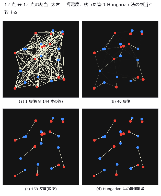
↑ 完全 2 部グラフ 144 本、ユークリッド長。
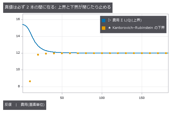
↑ 円盤 → 2 円盤。
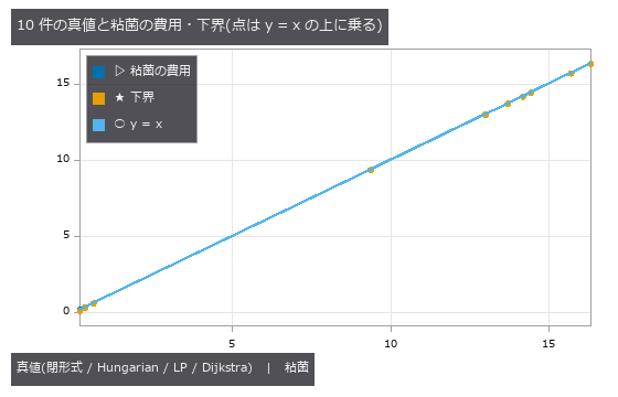
↑ 木 seed 0 16.34; 木 seed 1 13.71; 木 seed 2 14.19; 木 seed 3 15.71; 木 seed 4 14.44; 1 次元 0.3165; 割当 12×12 0.1632; 格子 6×6 LP 0.5918; 平行移動 (5, 8) 13; 単一対 7×…
py -3.11 examples/poc_physarum_transport.py
Source: examples/poc_physarum_transport.py
This run produced 5 figures in total - see them all
Ops used (notes): graph_physarum_transport · physarum_transport_image · wasserstein_1d
No.2026.154 —— Grading Skeleton Measurement on Real Trees — NeuroMorpho SWC as Ground Truth, and What Projection Breaks
The vessel-network PoC used a synthetic tree as truth; here the truth is a real tree — NeuroMorpho.Org SWC files (coordinates, radius and parent id per node; three mouse neocortical neurons, CC BY 4.0). SWC carries structural constraints (exactly one root, parent id < child id, nodes = edges + 1) that are gates in themselves: a broken tree is not graded. The 3-D Sholl count (intersections of branches with spheres around the soma) depends only on distances from the origin, so across 12 rotations not a single integer moves. Image measurement, however, runs on a projection — the projected Sholl count moves by up to 9–16 intersections with viewing angle, and the bifurcation count against ground truth 16 / 11 / 37 becomes 22–28 / 15–24 / 41–49 over 12 viewing angles (the excess is branch crossings that thinning turns into junctions), while skeleton length shrinks to 0.72–0.82 of the cable length. The precision of a “tree measurement” is set by the line of sight, not the tree. No data is bundled; without it the example runs on a synthetic tree that satisfies the same constraints (a tangled 3-D synthetic tree projects worse than the real ones — and says so).
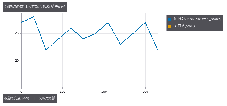
↑ Grading Skeleton Measurement on Real Trees — NeuroMorpho SWC as Ground Truth, and What Projection Breaks ―― The vessel-network PoC used a synthetic tree as truth; here the truth is a real tree — NeuroMorpho.Org SWC files (coordinates, radius and parent id per node; three mouse neocortical neurons, CC BY 4.0). SWC carries structural constraints (exactly one root, parent id < child id, nodes = edges + 1) that are gates in themselves: a broken tree is not graded. The 3-D Sholl count (intersections of branches with spheres around the soma) depends only on distances from the origin, so across 12 rotations not a single integer moves. Image measurement, however, runs on a projection — the projected Sholl count moves by up to 9–16 intersections with viewing angle, and the bifurcation count against ground truth 16 / 11 / 37 becomes 22–28 / 15–24 / 41–49 over 12 viewing angles (the excess is branch crossings that thinning turns into junctions), while skeleton length shrinks to 0.72–0.82 of the cable length. The precision of a “tree measurement” is set by the line of sight, not the tree. No data is bundled; without it the example runs on a synthetic tree that satisfies the same constraints (a tangled 3-D synthetic tree projects worse than the real ones — and says so).
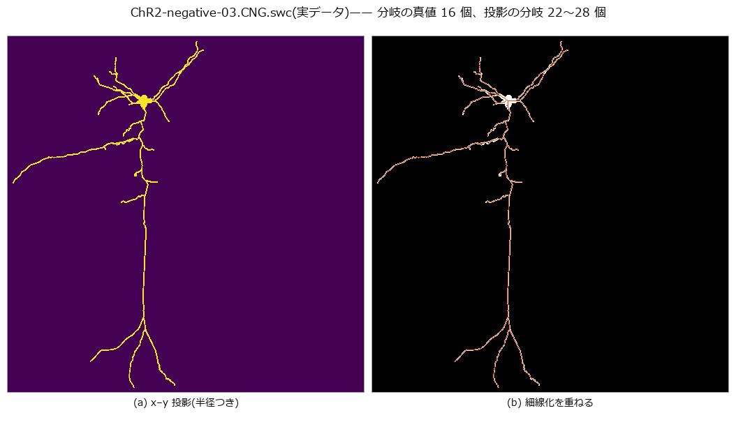
↑ The measurement (figure labels are in Japanese; the numbers are the same)
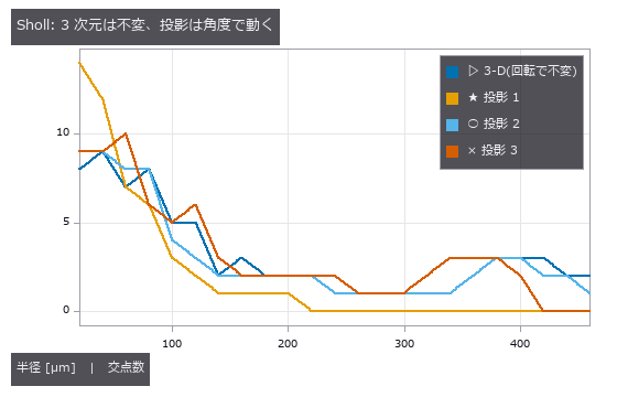
↑ 3-D の交点数は 12 回転で整数が 1 つも動かない。
py -3.11 examples/poc_swc_tree_truth.py
Source: examples/poc_swc_tree_truth.py
This run produced 3 figures in total - see them all
Ops used (notes): skeleton · tree_from_swc · tree_morphometry · tree_sholl
No.2026.164 —— The Worm Brain’s Core Is There from Birth — Counting the Cells That Stay in the Deepest Shell Across 8 Developmental Stages
The chemical-synapse wirings of Witvliet 2021’s 8 animals (0 h after birth → adult) are peeled with three new ops: graph_kcore (k-core / weighted s-core; in, out, total, undirected), graph_rich_club_curve (the rich-club coefficient for every k, divided by the degree-preserving null) and graph_core_persistence (the cells that stay in the deepest shell of all K animals). Gates are theorems: a complete graph is one shell of index n − 1, a tree 1, a cycle 2; the s-core of a 0/1 matrix equals the k-core exactly; weights × c → indices × c; the undirected k-core agrees with networkx on every node; φ(k) equals the single-k graph_rich_club for every k. Peeled by synapse count, the deepest (in-degree s-core) shell stays at 6–10 cells through development while its index deepens from 7 to 55, and the interneuron pair RIA is in the deepest shell of all 8 (10 motor and 2 interneuron classes; no muscle or glia). Peeled by 0/1, the k-core is coarse even in the adult (index 3–5) and its deepest shell swells to 150 cells. 51 cells persist in at least one of the 4 core types (in / out × k / s) — the published value of Yadav & Singh 2026 (bioRxiv); their ‘only AIBR, RIBL, RIAR among head neurons’ does not match the RIAL, RIAR persistent in all 4 types under my definition, and is recorded as is. A rich-club band exists at every stage (peak ratio 1.4–3.3, k = 1–28 in the adult). Figures: the 8 wirings on the neuron positions (skeleton roots, viewed along the body axis) aligned to the adult by Procrustes, and a moving figure interpolating between stages as connections grow and the core changes hands. ≈ 17 s.
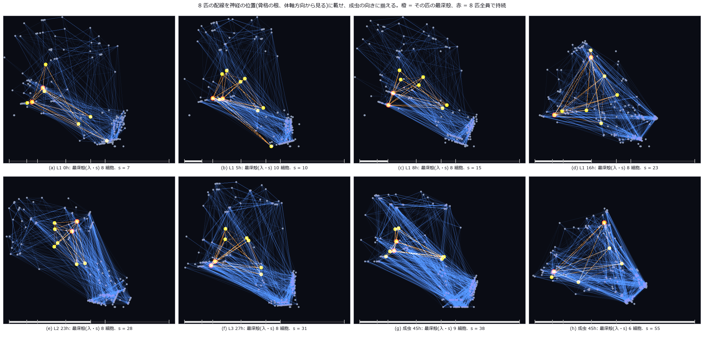
↑ The Worm Brain’s Core Is There from Birth — Counting the Cells That Stay in the Deepest Shell Across 8 Developmental Stages ―― The chemical-synapse wirings of Witvliet 2021’s 8 animals (0 h after birth → adult) are peeled with three new ops: graph_kcore (k-core / weighted s-core; in, out, total, undirected), graph_rich_club_curve (the rich-club coefficient for every k, divided by the degree-preserving null) and graph_core_persistence (the cells that stay in the deepest shell of all K animals). Gates are theorems: a complete graph is one shell of index n − 1, a tree 1, a cycle 2; the s-core of a 0/1 matrix equals the k-core exactly; weights × c → indices × c; the undirected k-core agrees with networkx on every node; φ(k) equals the single-k graph_rich_club for every k. Peeled by synapse count, the deepest (in-degree s-core) shell stays at 6–10 cells through development while its index deepens from 7 to 55, and the interneuron pair RIA is in the deepest shell of all 8 (10 motor and 2 interneuron classes; no muscle or glia). Peeled by 0/1, the k-core is coarse even in the adult (index 3–5) and its deepest shell swells to 150 cells. 51 cells persist in at least one of the 4 core types (in / out × k / s) — the published value of Yadav & Singh 2026 (bioRxiv); their ‘only AIBR, RIBL, RIAR among head neurons’ does not match the RIAL, RIAR persistent in all 4 types under my definition, and is recorded as is. A rich-club band exists at every stage (peak ratio 1.4–3.3, k = 1–28 in the adult). Figures: the 8 wirings on the neuron positions (skeleton roots, viewed along the body axis) aligned to the adult by Procrustes, and a moving figure interpolating between stages as connections grow and the core changes hands. ≈ 17 s.
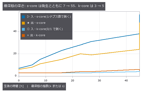
↑ The measurement ―― 同じ 8 匹。0/1 の k-core は成虫でも指数 5、最深殻が 179 細胞まで膨らむ。シナプス数で剥く s-core は最深殻が 6〜10 細胞のまま深くなる。 (figure labels are in Japanese; the numbers are the same)
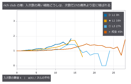
↑ 次数保存ヌル 20 標本。
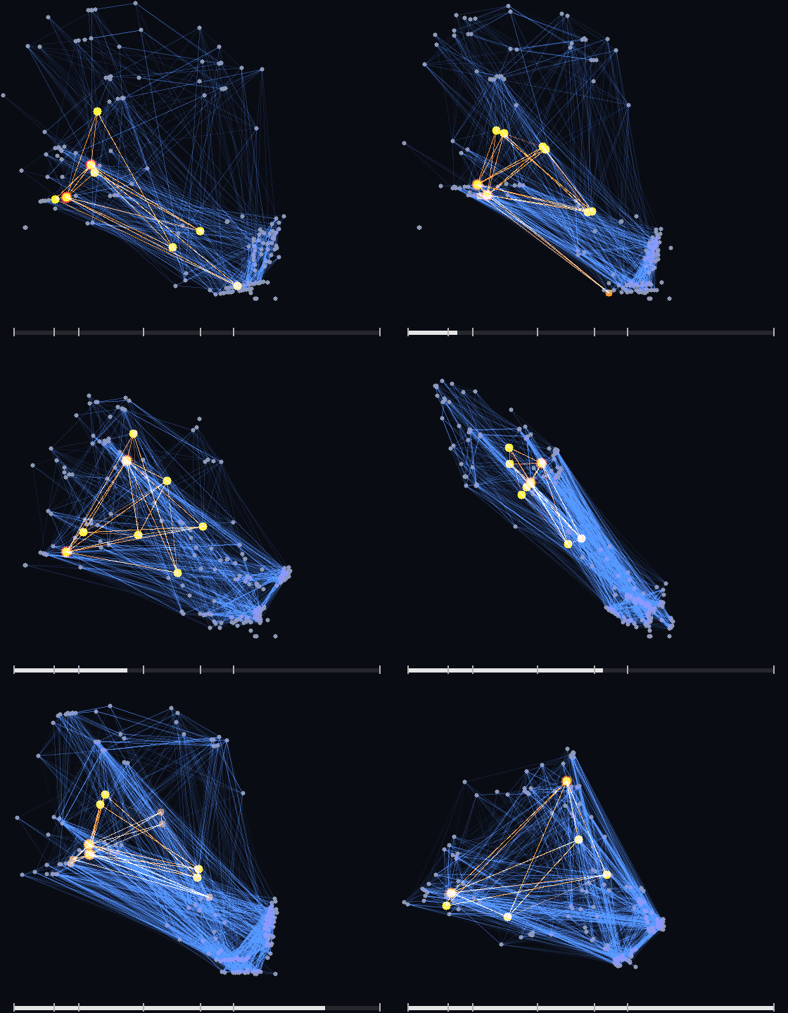
↑ The animation ―― 生後 0 時間から成虫まで。結合が生え、最深殻(橙)が入れ替わる中で、赤の細胞(RIAL RIAR)は一度も外れない。
py -3.11 examples/poc_worm_core_persists.py
Source: examples/poc_worm_core_persists.py
This run produced 4 figures in total - see them all
Ops used (notes): graph_core_persistence · graph_kcore · graph_rich_club · graph_rich_club_curve
No.2026.260 —— Drawing the Male Fly Brain as 126,104 Cell Bodies — A New Point-Cloud Renderer, Scored Against Four Answers from Outside the Picture
From the MaleCNS v1.0 annotations (Janelia FlyEM × Google Research, the whole male CNS, CC BY 4.0) the positions and superclasses of 126,104 brain cell bodies (VNC and ascending excluded) are drawn as a point cloud from the front, side and top and in rotation (optic-lobe intrinsic 81,055, central-brain intrinsic 31,997, visual projection 9,162, descending 1,308, …). Fullseye had no op that turns a point cloud into a colour picture; the brain on the back of the ViEW 2026 business card was placed point by point in hand-written numpy. The new op points_render (ops3d / render) splats sub-pixel footprints (gaussian / disc / point) and either alpha-composites them in depth order or adds them conserving the total light. The gates use values the renderer never computes: 99.5 % of the cell bodies labelled L land in the right half of the front view (seen from the front the fly’s left is on the right); 4,050 Kenyon cells picked by type name sit dorsal and posterior of 437 antennal-lobe neurons; the column sums of the front and top views (two different cameras) agree mirrored to 1.8e-15; the additive image sums to the point count within 1.2e-16; each class’s image centroid lies on the closed-form projection within 1.4e-5 px. The op has 37 unit gates (its z-buffer matches render_point_depth on every pixel; a quarter turn about the axis equals numpy.rot90), and ten deliberate breakages (no depth sort, half-pixel shift, transposed rotation, transmittance off by one, …) all turn them red. Cutting the Gaussian at 3 sigma moved centroids by 0.017 px and a circular cut made column sums depend on the row by 1e-5; the cut is now 4 sigma per axis. Raw data is never committed (cached from local feather files; without them a synthetic brain runs the same gates and the recorded values are printed).
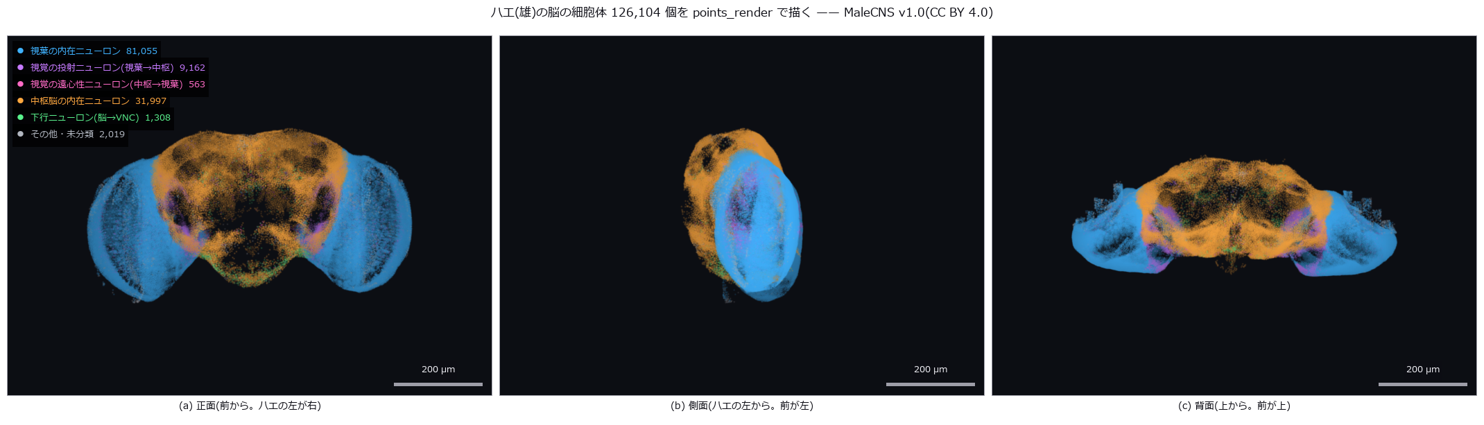
↑ Drawing the Male Fly Brain as 126,104 Cell Bodies — A New Point-Cloud Renderer, Scored Against Four Answers from Outside the Picture ―― From the MaleCNS v1.0 annotations (Janelia FlyEM × Google Research, the whole male CNS, CC BY 4.0) the positions and superclasses of 126,104 brain cell bodies (VNC and ascending excluded) are drawn as a point cloud from the front, side and top and in rotation (optic-lobe intrinsic 81,055, central-brain intrinsic 31,997, visual projection 9,162, descending 1,308, …). Fullseye had no op that turns a point cloud into a colour picture; the brain on the back of the ViEW 2026 business card was placed point by point in hand-written numpy. The new op points_render (ops3d / render) splats sub-pixel footprints (gaussian / disc / point) and either alpha-composites them in depth order or adds them conserving the total light. The gates use values the renderer never computes: 99.5 % of the cell bodies labelled L land in the right half of the front view (seen from the front the fly’s left is on the right); 4,050 Kenyon cells picked by type name sit dorsal and posterior of 437 antennal-lobe neurons; the column sums of the front and top views (two different cameras) agree mirrored to 1.8e-15; the additive image sums to the point count within 1.2e-16; each class’s image centroid lies on the closed-form projection within 1.4e-5 px. The op has 37 unit gates (its z-buffer matches render_point_depth on every pixel; a quarter turn about the axis equals numpy.rot90), and ten deliberate breakages (no depth sort, half-pixel shift, transposed rotation, transmittance off by one, …) all turn them red. Cutting the Gaussian at 3 sigma moved centroids by 0.017 px and a circular cut made column sums depend on the row by 1e-5; the cut is now 4 sigma per axis. Raw data is never committed (cached from local feather files; without them a synthetic brain runs the same gates and the recorded values are printed).
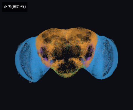
↑ The measurement ―― 回転の 1 コマ目(静止画の代わり)。正面から見たところ。MaleCNS v1.0(CC BY 4.0) (figure labels are in Japanese; the numbers are the same)
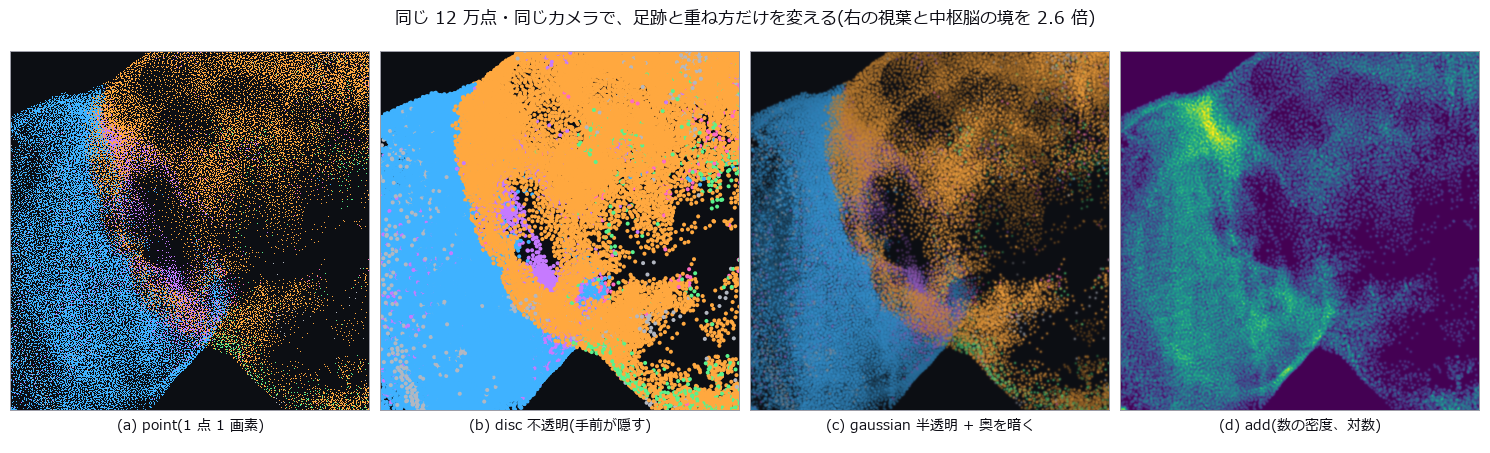
↑ points_render のノブ: footprint(point / disc / gaussian)と composite(over / add)。
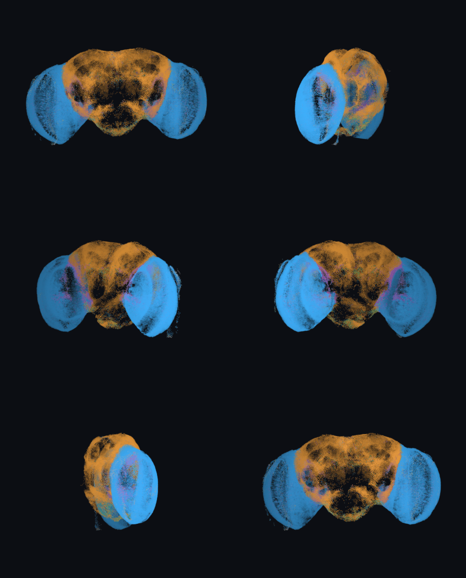
↑ The animation ―― 背腹の軸まわりに 1 周(36 コマ)。どのコマも points_render の 1 回の呼び出し。MaleCNS v1.0(CC BY 4.0)
py -3.11 examples/poc_flybrain_pointcloud.py
Source: examples/poc_flybrain_pointcloud.py
This run produced 4 figures in total - see them all
Ops used (notes): annotate_figure_grid · annotate_scale_bar · gaussian · points_render · text_box
The Astronomy and Environment Wing — Biased by Position, Flipped by the Definition of Truth
Stellar brightness and position, the solar limb, all-sky cloud cover, sea-ice concentration, crop cover, terrain, river stage. The subjects are far away and ground truth is normally out of reach. The 21 exhibits here turn that around, placing their truth in closed forms and public data: celestial coordinates, the solid angle of a spherical cap, Eddington limb darkening, elevation tiles from the Geospatial Information Authority of Japan.
The shared finding is that the same object reads differently depending on where it is: the same cloud counts 1.45x more at the horizon than at the zenith; clouds of equal optical thickness are detected or not depending on their angular distance from the sun; the same reflection makes one detector read quietly low and another stop silently.
The other is that the definition of truth decides the conclusion. Counting thin ice as ‘ice’ or not sends the same estimate to -4.4 or +2.7 points; a cloud fraction reported without its horizon-mask angle can legitimately claim anything from 0.18 to 0.23. What you call the truth has to be written down before the instrument is.
No.2026.001 —— All-Sky Cloud Cover — Counting Pixels Is Biased by Position
One cloud occupies different pixel areas at different positions in an all-sky image. Spherical caps were projected through a fisheye model and counted out to a zenith angle of 82 degrees. Pixel counting increasingly overstates clouds near the horizon, while geometric and detection errors partly cancel.
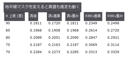
↑ All-Sky Cloud Cover — Counting Pixels Is Biased by Position ―― Spherical-cap clouds (closed-form solid angle) placed in an equidistant fisheye sky, with cloud fraction counted by pixel ratio and by solid-angle weight. The same cloud reads 0.00789 at the zenith and 0.01142 at 82 degrees (1.45x). Geometry alone errs by -5.02 %, detection alone by +37.95 %, and the naive count cancels them to +29.73 %.
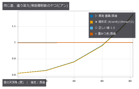
↑ The measurement ―― 画素数比は天頂で 0.81、地平線側で 1.17。重みを掛けると 1 に張り付く。 (figure labels are in Japanese; the numbers are the same)
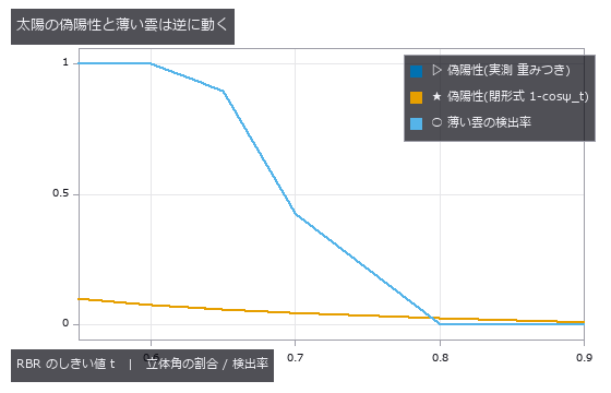
↑ 偽陽性は実測と閉形式が重なる。
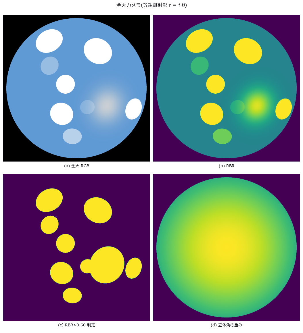
↑ 4 枚目が sinθ/θ。
py -3.11 examples/poc_allsky_cloud_cover.py
Source: examples/poc_allsky_cloud_cover.py
This run produced 4 figures in total - see them all
Ops used (notes): equirect_from_fisheye_pair · polar_trans_image
No.2026.002 —— How Many Frames for What Photometric Precision?
The question is whether stacking more star fields reduces photometric error at the theoretical rate. Fields with known stellar brightness were stacked until aperture-photometry error fell to 0.1616 %. The expected improvement appears, while rejection averaging stays closer to truth when a cosmic ray is present.
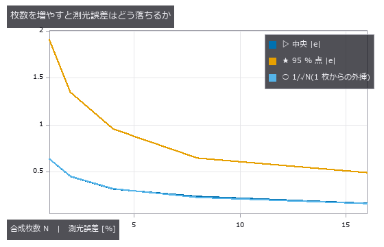
↑ How Many Frames for What Photometric Precision? ―― A star field placed to specification and stacked N deep, to see whether aperture-photometry error falls as 1/√N. From N = 1 to 16 the median error drops from 0.6350 % to 0.1616 %, within 4.6 % of theory in all eight cases. One cosmic ray pushes the plain mean to +5.89 % while κ-σ clipping holds +0.30 %; the rejection rate does not move, so ‘the rejection rate went up, therefore it worked’ is not an available argument.
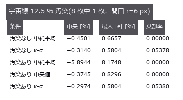
↑ The measurement ―― 単純平均だけが 5.9 % 残る。κ-σ は汚染なしと区別できないところまで戻すが、棄却率はほとんど動かない。 (figure labels are in Japanese; the numbers are the same)
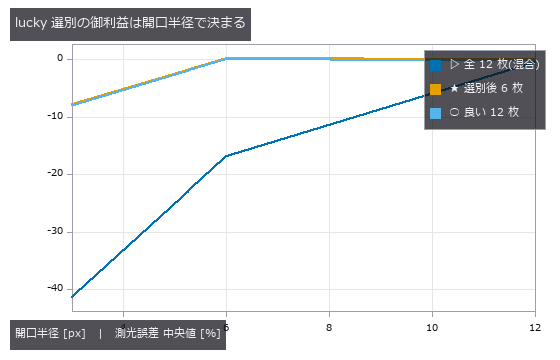
↑ 開口を広く取れるなら、ぼけたフレームも同じ明るさを持っている(r=12 では 3 本が重なる)。
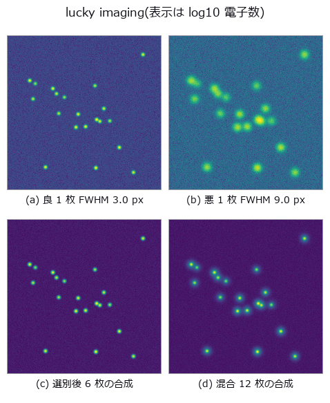
↑ 悪いほうは星が広がっている。
py -3.11 examples/poc_astro_photometry.py
Source: examples/poc_astro_photometry.py
This run produced 4 figures in total - see them all
Ops used (notes): aperture_photometry · drizzle_resample · lucky_select · median · sigma_clip_stack · synth_frame_series · synth_starfield
No.2026.059 —— Change detection under misregistration — false positives are edge bands, with a cliff
In two-date subtraction, unchanged edges can appear as change solely from misregistration. Known land changes were inserted before shifting the images, revealing a false-positive cliff at 0.5 px. Residual alignment error follows the same cliff, which radiometric correction cannot remove.

↑ Change detection under misregistration — false positives are edge bands, with a cliff ―― A two-date synthetic land surface (fields, roads, buildings, forest, lake) with planted changes (new buildings, clear-cut, lake expansion); date 2 is degraded by sub-pixel shift, small rotation and an illumination change, and the false-positive area of plain differencing is measured. False positives stay at the noise floor up to 0.3 px and jump at 0.5 px (matching the PSF-derived onset δ=τσ√2π/C=0.351 px), reaching 7175 px at 3 px. The edge-length × shift rule gives 0.78× at 3 px but cannot explain the cliff; the PSF+noise edge-ledger prediction is within 0.84–1.07×. Three registration paths (PIV, keypoints, LK) bring the residual down to 0.02–0.13 px, but the only phase-correlation path is 3-D and integer-valued (residual 0.72 px), and its 995 px of false positives lands on the shift-only sweep read at the same residual (915 px). Clear-cut recall is 0.33 even with perfect alignment; the illumination-only 17198 px vanish with radiometric normalisation while the 3497 px from shift do not.*
Terms: PSF — The spatial response of an imaging system to a point object, describing how that point is blurred in the image.

↑ The measurement ―― 0.35 px までゼロ、そこから立ち上がる。比例則は崖を説明しない。 (figure labels are in Japanese; the numbers are the same)

↑ この回の図

↑ 回転 1 度の偽陽性地図(橙)。

↑ この回の図
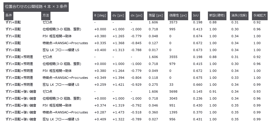
↑ この回の図
py -3.11 examples/poc_change_detection_misreg.py
Source: examples/poc_change_detection_misreg.py
This run produced 11 figures in total - see them all
Ops used (notes): affine_trans_image · histogram_match · match_phase_3d · opening_circle · piv_cross_correlate · piv_outlier_mask · procrustes_fit · threshold · voxel_iou
No.2026.096 —— A 3-D Thermal Field from Sparse Sensors — The Grid’s Blind Spot Erases a Rack
A temperature field for a 12 x 8.4 x 3.0 m server room is written as a formula, then reconstructed from a grid of temperature sensors to find three overloaded racks. The null baseline, the mean of all sensors spread over the whole room, gives an RMSE of 2.192 degrees and finds no hot spot at all; the best method, a thin-plate RBF, gives 0.214, ten times better. The cliff can be stated in closed form before measuring: on a grid of spacing d the point furthest from a peak is the cell centre at dsqrt(3)/2, so a Gaussian of width sigma is recovered at exp(-3d^2/8sigma^2) and halves at d = 1.3596 sigma. Isolating the geometry, prediction and measurement differ by at most 1.2e-15. What failed was not the formula but the quantity a site can actually measure: the peak of a reconstructed field carries the background’s reconstruction error at the same place, so a naive measurement exceeds the prediction by up to +0.2598 and the cliff looks shallower than it is. The sigma=0.22 m rack is recovered at 0.000014 at d=1.20 m, effectively gone, yet naively appears to hold 0.1609 — what remains is the background error. The closed form is a floor, not a curve: at the same d=0.60 m, recovery jumps from 0.0615 at a cell centre to 1.0 directly above a sensor, so only the worst phase is usable for design. Random placement does not remove blind spots; it only reshuffles which rack falls into one. Measured, 6.17 % of random points exceed the grid’s worst distance against a Poisson prediction of 6.58 %. The grid never breaks its geometric lower bound while random placement broke it for two of the three racks: with the same sensor count, only one of them supports a guarantee. Swapping the interpolator moves the coefficient, not the exponent — all three slopes of log recovery against d^2 sit within 3.05 % of the predicted -3.0612 — but the prediction that the cliff position is method-independent was wrong: the thin-plate spline overshoots its own nodes by a factor of 1.372 and shifts the half-recovery spacing from 0.4777 to 0.6015 m, a 26 % move. The follow-up prediction, that an overshooting method raises the false peaks by the same factor, was also wrong: the nearest-neighbour floor is 0.975 degrees, 6.5 times the sensor noise, because a staircase approximation of a smooth background is itself a step. No method wins all three rulers at once, and at d=1.20 m linear interpolation falls outside the convex hull for 71.2 % of the evaluation points, silently becoming nearest-neighbour at the walls. The gap this PoC found has since been filled: fs.interp_scattered interpolates a field from scattered N-D points and returns the fraction of query points that fell outside the convex hull — the 71.2 % measured here is exactly the quantity that would otherwise turn silently into NaN or into another method under the first method’s name.
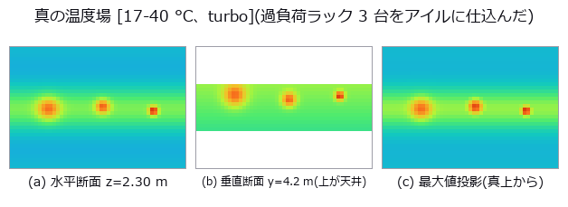
↑ A 3-D Thermal Field from Sparse Sensors — The Grid’s Blind Spot Erases a Rack ―― A temperature field for a 12 x 8.4 x 3.0 m server room is written as a formula, then reconstructed from a grid of temperature sensors to find three overloaded racks. The null baseline, the mean of all sensors spread over the whole room, gives an RMSE of 2.192 degrees and finds no hot spot at all; the best method, a thin-plate RBF, gives 0.214, ten times better. The cliff can be stated in closed form before measuring: on a grid of spacing d the point furthest from a peak is the cell centre at dsqrt(3)/2, so a Gaussian of width sigma is recovered at exp(-3d^2/8sigma^2) and halves at d* = 1.3596 sigma. Isolating the geometry, prediction and measurement differ by at most 1.2e-15. What failed was not the formula but the quantity a site can actually measure: the peak of a reconstructed field carries the background’s reconstruction error at the same place, so a naive measurement exceeds the prediction by up to +0.2598 and the cliff looks shallower than it is. The sigma=0.22 m rack is recovered at 0.000014 at d=1.20 m, effectively gone, yet naively appears to hold 0.1609 — what remains is the background error. The closed form is a floor, not a curve: at the same d=0.60 m, recovery jumps from 0.0615 at a cell centre to 1.0 directly above a sensor, so only the worst phase is usable for design. Random placement does not remove blind spots; it only reshuffles which rack falls into one. Measured, 6.17 % of random points exceed the grid’s worst distance against a Poisson prediction of 6.58 %. The grid never breaks its geometric lower bound while random placement broke it for two of the three racks: with the same sensor count, only one of them supports a guarantee. Swapping the interpolator moves the coefficient, not the exponent — all three slopes of log recovery against d^2 sit within 3.05 % of the predicted -3.0612 — but the prediction that the cliff position is method-independent was wrong: the thin-plate spline overshoots its own nodes by a factor of 1.372 and shifts the half-recovery spacing from 0.4777 to 0.6015 m, a 26 % move. The follow-up prediction, that an overshooting method raises the false peaks by the same factor, was also wrong: the nearest-neighbour floor is 0.975 degrees, 6.5 times the sensor noise, because a staircase approximation of a smooth background is itself a step. No method wins all three rulers at once, and at d=1.20 m linear interpolation falls outside the convex hull for 71.2 % of the evaluation points, silently becoming nearest-neighbour at the walls. The gap this PoC found has since been filled: fs.interp_scattered interpolates a field from scattered N-D points and returns the fraction of query points that fell outside the convex hull — the 71.2 % measured here is exactly the quantity that would otherwise turn silently into NaN or into another method under the first method’s name.*
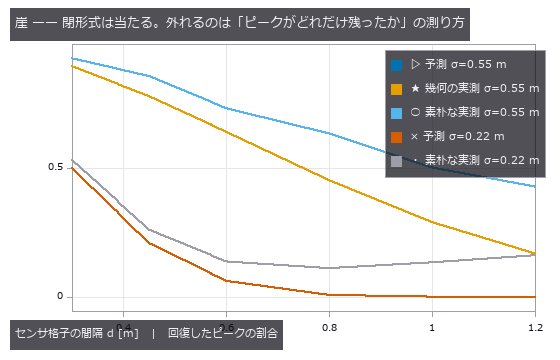
↑ The measurement ―― 幾何の実測は予測と最大 1.2e-15 しか違わない。素朴な実測が上に浮くぶんが背景の復元誤差。 (figure labels are in Japanese; the numbers are the same)
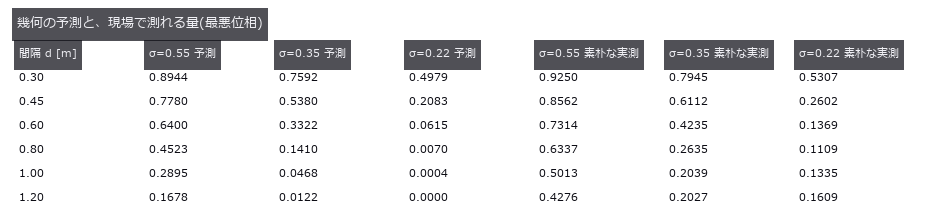
↑ この回の図

↑ 格子の最悪距離 0.520 m を乱数の 6.17 % が超えた(予測 6.58 %)。
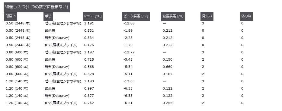
↑ この回の図
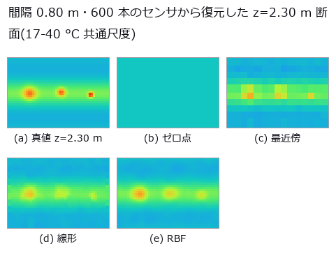
↑ 横=x 0..12 m、縦=y 0..8.4 m。
py -3.11 examples/poc_datacenter_thermal_field.py
Source: examples/poc_datacenter_thermal_field.py
This run produced 8 figures in total - see them all
Ops used (notes): interp_scattered · render_volume_projection · rmse · vol_local_maxima
No.2026.012 —— Measuring Terrain — Slope, Flow and Insolation Against Closed Forms
Slope, curvature and sky-view factor checked against closed forms on a plane, a cone and a Gaussian hill. Halving the cell size cuts the hill’s curvature error by about four — a discretisation error, not a wrong formula. The sky-view factor takes 2.03 s on a 513×513 grid with 8 directions; before the rewrite it took 41.9 s, and the tests had only ever checked that it runs.
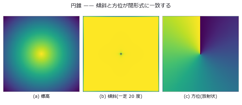
↑ Measuring Terrain — Slope, Flow and Insolation Against Closed Forms ―― Slope, curvature and sky-view factor checked against closed forms on a plane, a cone and a Gaussian hill. Halving the cell size cuts the hill’s curvature error by about four — a discretisation error, not a wrong formula. The sky-view factor takes 2.03 s on a 513×513 grid with 8 directions; before the rewrite it took 41.9 s, and the tests had only ever checked that it runs.
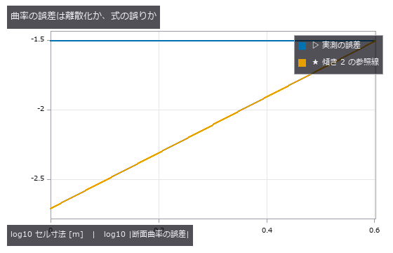
↑ The measurement ―― 参照線と平行 = 2 次収束 = 離散化の誤差。式が違えばセルを細かくしても誤差は下げ止まる。 (figure labels are in Japanese; the numbers are the same)
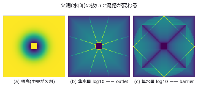
↑ 同じ地形・同じ op。
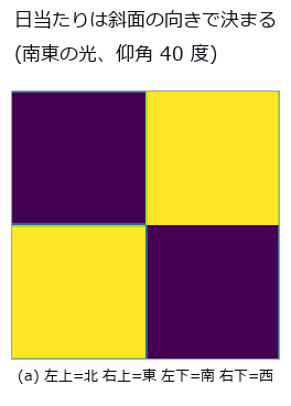
↑ 陰影の平均は 北向き 0.354 / 東向き 0.811 / 南向き 0.811 / 西向き 0.354。
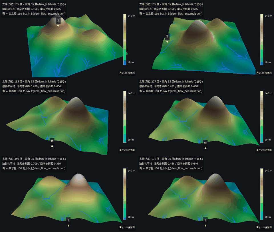
↑ The animation ―― 主図(動画、640 × 360・30 fps・11 秒): 800 m 四方の地形(セル 5 m)を南南西から北へ回り込み、止まって太陽を一周させる。陰影は描画の光でなく dem_hillshade(仰角 35 度)の出力で塗り、青は dem_flow_accumulation の集水量 150 セル以上。南向き斜面の陰影の平均は太陽方位 187 度で最大 0.719、北向き斜面は 1 度で最大 0.709 —— 日当たりは斜面の向きで決まる(§6 の平面と同じ結論)。高さは画面上だけ 2.5 倍。
py -3.11 examples/poc_dem_terrain.py
Source: examples/poc_dem_terrain.py
This run produced 5 figures in total - see them all
Ops used (notes): color_bar · dem_aspect · dem_curvature · dem_fill_sinks · dem_flow_accumulation · dem_hillshade · dem_sky_view_factor · dem_slope · text_box
No.2026.066 —— Exoplanet transit from aperture photometry — depth and duration fail separately
A synthetic star field (240 frames) carries a 10 ppt limb-darkened transit on the target only, with transparency variation, sub-pixel drift, flat-field non-uniformity and photon noise injected from separate random streams; fullseye’s star_detect → frame_align → aperture_photometry extracts the light curve. The zero point (target aperture sum alone) breaks under clouds to a depth error of +72 ppt; the ratio to comparison stars gives -0.13 ppt / T14 -0.9 fr. Comparison-star choice moves the residual rms from 1.91 to 11.43 ppt (6.0x), and inverse-variance weights computed from raw variance are fooled by clouds into 1.52x worse than a plain sum. The small-aperture cliff at 1σ was not the predicted centroid error but the op’s aperture-mask staircase (supersample=8: a static star sits 1.69x above theory, 0.93x at 32). The SNR=5 detection limit is 1.48 ppt measured vs 1.45 ppt theory with a known ephemeris, 2.0 ppt blind, where the duration breaks before the depth. Drift 2 px and a 3 % flat are harmless alone (0.16 / 0.08 ppt) but multiply into a 0.94 ppt false depth, 2.97 ppt (30 % of truth) at 4 px.
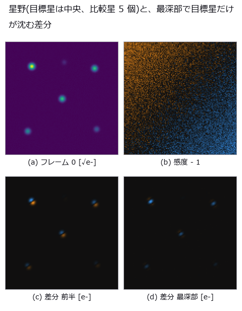
↑ Exoplanet transit from aperture photometry — depth and duration fail separately ―― A synthetic star field (240 frames) carries a 10 ppt limb-darkened transit on the target only, with transparency variation, sub-pixel drift, flat-field non-uniformity and photon noise injected from separate random streams; fullseye’s star_detect → frame_align → aperture_photometry extracts the light curve. The zero point (target aperture sum alone) breaks under clouds to a depth error of +72 ppt; the ratio to comparison stars gives -0.13 ppt / T14 -0.9 fr. Comparison-star choice moves the residual rms from 1.91 to 11.43 ppt (6.0x), and inverse-variance weights computed from raw variance are fooled by clouds into 1.52x worse than a plain sum. The small-aperture cliff at 1σ was not the predicted centroid error but the op’s aperture-mask staircase (supersample=8: a static star sits 1.69x above theory, 0.93x at 32). The SNR=5 detection limit is 1.48 ppt measured vs 1.45 ppt theory with a known ephemeris, 2.0 ppt blind, where the duration breaks before the depth. Drift 2 px and a 3 % flat are harmless alone (0.16 / 0.08 ppt) but multiply into a 0.94 ppt false depth, 2.97 ppt (30 % of truth) at 4 px.
[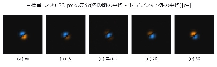](https://raw.githubusercontent.com/furuse-kazufumi/fullseye/master/docs/articles/assets/poc/poc_exoplanet_transit/02_frames_transit_phases.png)
↑ The measurement ―― 前/入/最深部/出/後の各段階で平均した画像からトランジット外の平均を引いた [e-]。4 倍拡大 (figure labels are in Japanese; the numbers are the same)

↑ ゼロ点と比較星の和は雲(全星共通)そのもの。
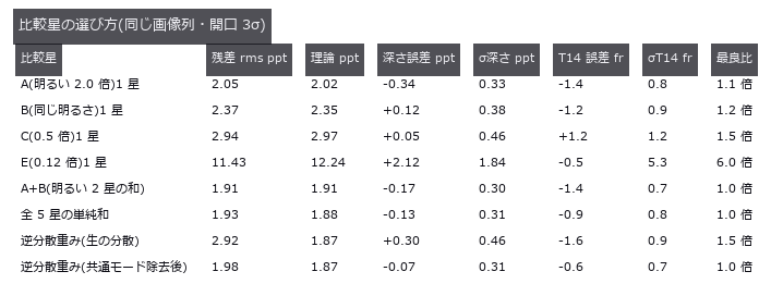
↑ この回の図
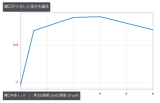
↑ この回の図
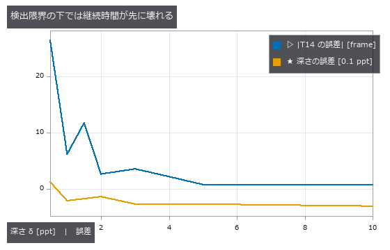
↑ この回の図
py -3.11 examples/poc_exoplanet_transit.py
Source: examples/poc_exoplanet_transit.py
This run produced 11 figures in total - see them all
Ops used (notes): aperture_photometry · frame_align · normalize · sigma_clip_stack · star_detect
No.2026.098 —— Coordinates Go Wrong by Tens of Metres While Still Looking Plausible
| GNSS returns an ellipsoidal height; maps and drawings use an orthometric one, and the two differ by the geoid undulation — 30 to 40 m around Japan. This exhibit plants a synthetic geoid field and measures which quantities that confusion reaches and which ones it cancels out of. The floor is taken twice: the round trip of the existing operators closes to 1.07e-06 m, and an independent iterative implementation agrees to 7.2e-07 m in latitude — because a round trip alone cannot rule out both directions being wrong the same way. Several closed forms landed: the bound on slope error, atan | grad N | , predicted 0.008771 degrees against 0.008600 measured, with the constant-undulation control at 2.0e-14 degrees, which is exactly zero; the volume error A times the mean undulation agreed to 1.5e-08 cubic metres; the fraction of flat ground whose flow direction reverses was predicted at 76.1 % and measured at 76.2 %. One prediction was badly wrong: the bound on line-of-sight clearance was set at 2.60 m and measured 0.052 m, fifty times smaller, because the linear part of the undulation rides on the sight line and the ground equally and cancels; Earth curvature matters 276 times more. The flat-earth cliff has a closed form but not a single number — at 10 km the prediction of -7.8481 m brackets measurements of -7.8652 m north-south and -7.8303 m east-west, the difference between the meridional and prime-vertical radii. The theme is that the same 36 m is everything or nothing depending on the quantity: it nearly vanishes from differences and survives whole in absolutes, changing an earthwork volume by 3.97e+07 cubic metres and a flooded area from 41.9 % to zero. A control where the design surface is built from the same GNSS shows zero error — a contaminated ruler applied to a contaminated object hides the error. A datum mix-up shifts positions by 446.6 m on average while a relative check between baselines shows only 0.106 m per kilometre, four thousand times less; the danger is not the size but the plausibility. Counting quiet failures against loud ones over a 3600-point global grid, the only mistake that raises is swapping latitude and longitude, and only half the time; radians-for-degrees, a flipped longitude sign, swapped ECEF axes (whose results land in a valid latitude and longitude range 100 % of the time) and feet-for-metres all pass silently. Ten of eleven entries fail quietly. Along the way a real defect was found and fixed: near the Earth’s centre the ECEF-to-geodetic conversion returned a latitude of 180 degrees — a value that does not exist, and one its own inverse rejects. |
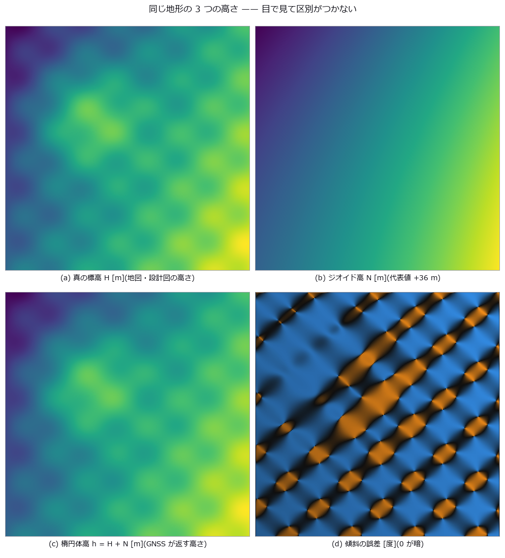
| *↑ Coordinates Go Wrong by Tens of Metres While Still Looking Plausible ―― GNSS returns an ellipsoidal height; maps and drawings use an orthometric one, and the two differ by the geoid undulation — 30 to 40 m around Japan. This exhibit plants a synthetic geoid field and measures which quantities that confusion reaches and which ones it cancels out of. The floor is taken twice: the round trip of the existing operators closes to 1.07e-06 m, and an independent iterative implementation agrees to 7.2e-07 m in latitude — because a round trip alone cannot rule out both directions being wrong the same way. Several closed forms landed: the bound on slope error, atan | grad N | , predicted 0.008771 degrees against 0.008600 measured, with the constant-undulation control at 2.0e-14 degrees, which is exactly zero; the volume error A times the mean undulation agreed to 1.5e-08 cubic metres; the fraction of flat ground whose flow direction reverses was predicted at 76.1 % and measured at 76.2 %. One prediction was badly wrong: the bound on line-of-sight clearance was set at 2.60 m and measured 0.052 m, fifty times smaller, because the linear part of the undulation rides on the sight line and the ground equally and cancels; Earth curvature matters 276 times more. The flat-earth cliff has a closed form but not a single number — at 10 km the prediction of -7.8481 m brackets measurements of -7.8652 m north-south and -7.8303 m east-west, the difference between the meridional and prime-vertical radii. The theme is that the same 36 m is everything or nothing depending on the quantity: it nearly vanishes from differences and survives whole in absolutes, changing an earthwork volume by 3.97e+07 cubic metres and a flooded area from 41.9 % to zero. A control where the design surface is built from the same GNSS shows zero error — a contaminated ruler applied to a contaminated object hides the error. A datum mix-up shifts positions by 446.6 m on average while a relative check between baselines shows only 0.106 m per kilometre, four thousand times less; the danger is not the size but the plausibility. Counting quiet failures against loud ones over a 3600-point global grid, the only mistake that raises is swapping latitude and longitude, and only half the time; radians-for-degrees, a flipped longitude sign, swapped ECEF axes (whose results land in a valid latitude and longitude range 100 % of the time) and feet-for-metres all pass silently. Ten of eleven entries fail quietly. Along the way a real defect was found and fixed: near the Earth’s centre the ECEF-to-geodetic conversion returned a latitude of 180 degrees — a value that does not exist, and one its own inverse rejects.* |
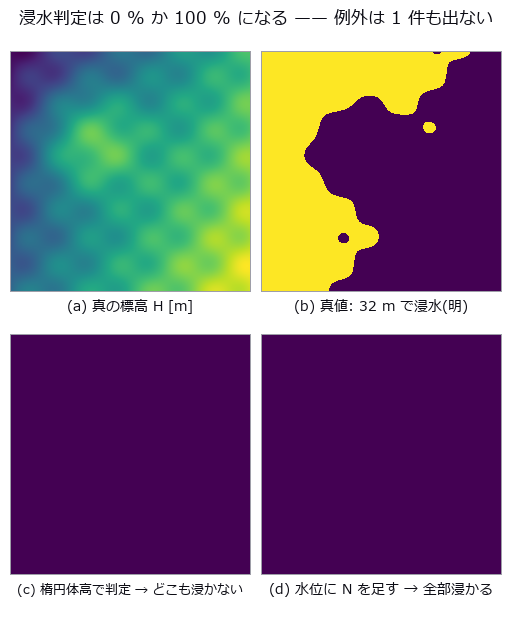
↑ The measurement ―― 分母 58081 セル。真値 24325(41.9 %)に対し、誤用は 0 と 58081。どちらの絵も「もっともらしい」(全面浸水は津波の図に見える)。 (figure labels are in Japanese; the numbers are the same)
| [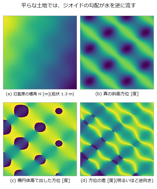](https://raw.githubusercontent.com/furuse-kazufumi/fullseye/master/docs/articles/assets/poc/poc_geodetic_height_frames/03_flow_flip.png) |
| *↑ 真の勾配の中央値 9.15e-05 に対し | ∇N | は 1.2e-04。* |
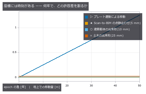
↑ 2.5 cm/年(代表値)。
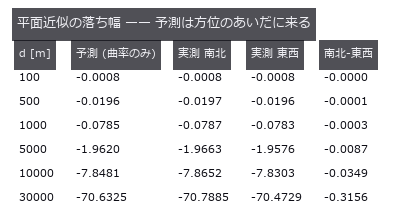
↑ 真の ECEF(dem_geodetic_to_ecef)を自前の ENU 回転に通して測った。

↑ 全球 3600 点。
py -3.11 examples/poc_geodetic_height_frames.py
Source: examples/poc_geodetic_height_frames.py
This run produced 13 figures in total - see them all
Ops used (notes): datum_tilt_check · dem_aspect · dem_datum_shift_3param · dem_earth_curvature_drop · dem_ecef_to_geodetic · dem_enu_from_geodetic · dem_flow_direction · dem_geodetic_from_enu · dem_geodetic_to_ecef · dem_geoid_height · dem_height_frame_convert · dem_slope · material_xray_attenuation · median · water_attenuation
No.2026.068 —— Leaf disease severity — colour axes survive the lighting; the grade is decided by the leaf mask and the edge convention
A closed-form leaf outline with lesions of known area, over soil, side lighting, clipped highlights and a shadow, gives ground truth for disease severity (lesion pixels / leaf pixels). A fixed threshold on the green channel (the zero point) is off by +65.2 pt with soil alone; cutting the leaf with the illuminant-projected G and the lesions with Lab a* lands at -0.8 pt on the standard scene. Illumination falloff up to 50 % does not move a, but clipped highlights produce only false positives for a (+12.6 pt at 20 % coverage, 0.0 false negatives) versus +2.0 pt for hue, which is invariant to added white. With a 4 px soft lesion edge, choosing the 25 % or 75 % opacity contour as the boundary alone shifts the severity by ±3.5 pt (predicted within 0.4 pt by Steiner’s formula), and of 40 images placed within ±3 pt of a grade boundary, 19-35 are misgraded on soil by every method — on black cloth with a brightness leaf mask, a fixed hue threshold misgrades 8.
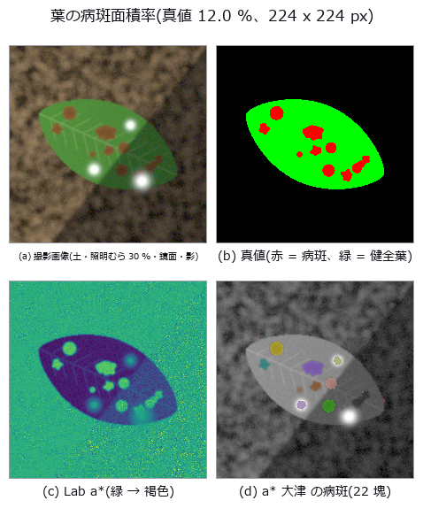
↑ Leaf disease severity — colour axes survive the lighting; the grade is decided by the leaf mask and the edge convention ―― A closed-form leaf outline with lesions of known area, over soil, side lighting, clipped highlights and a shadow, gives ground truth for disease severity (lesion pixels / leaf pixels). A fixed threshold on the green channel (the zero point) is off by +65.2 pt with soil alone; cutting the leaf with the illuminant-projected G and the lesions with Lab a lands at -0.8 pt on the standard scene. Illumination falloff up to 50 % does not move a, but clipped highlights produce only false positives for a (+12.6 pt at 20 % coverage, 0.0 false negatives) versus +2.0 pt for hue, which is invariant to added white. With a 4 px soft lesion edge, choosing the 25 % or 75 % opacity contour as the boundary alone shifts the severity by ±3.5 pt (predicted within 0.4 pt by Steiner’s formula), and of 40 images placed within ±3 pt of a grade boundary, 19-35 are misgraded on soil by every method — on black cloth with a brightness leaf mask, a fixed hue threshold misgrades 8.*

↑ The measurement ―― FN(青)の大きな塊は影と鏡面反射が重なった病斑(葉マスクごと落ちる)。FP(赤)は鏡面反射の下と病斑の縁。 (figure labels are in Japanese; the numbers are the same)
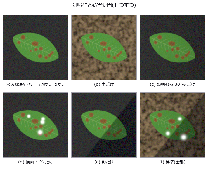
↑ この回の図
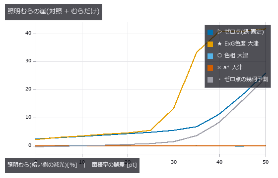
↑ ゼロ点は固定しきい値を葉が割る列から予測できる。

↑ 色相は白を足しても動かない(定義)。

↑ 予測の崖 1.8 px。
py -3.11 examples/poc_leaf_disease_area.py
Source: examples/poc_leaf_disease_area.py
This run produced 9 figures in total - see them all
Ops used (notes): access_channel · blob_features · blob_label · blob_overlay · fill_holes · gaussian · linear_to_srgb · plant_color_index · reg_close · reg_erode · rgb_to_lab · select_largest · sk_otsu · specular_free_transform · srgb_to_linear · trans_from_rgb
No.2026.106 —— Planting Known Stars in a Real Deep Field — Contamination Lies About the Measurement and the Confidence in the Same Direction
Gaussian stars of known flux planted in the real background of the Hubble Deep Field (NASA/STScI, public domain) — the truth is certain because it was planted, and only the background is real. The real sky is not Gaussian: a robust spread of 1,474 e- against a plain standard deviation of 6,698 e- (4.54x), so taking std for noise reports a detection limit 4.5 times too generous. The background is not one number either, ranging 3,176 to 8,448 e- across 195 tiles of 64x64, which leaves up to 3.6 sigma of systematic error after a single global subtraction. Even in the emptiest thirty per cent of the field a fixed amount leaks into the aperture: recovery runs 4.38x at F = 2,000 e- and 1.058x at 100,000, and it is an addition rather than a factor — 1 + C/(F·frac) fits all five points to within 0.9 %, with C = 6,677 e-, a mere 3.0 % of background times effective area. Predicting first that the bias falls below 10 % from 67,521 e- and then measuring there gives 1.086 against the predicted 1.100. In crowded positions the order of magnitude changes, 341x down to 7.80x: a median is robust to outliers, but when half the field is contaminated the median is the contamination. The confidence lies in the same direction — the op reports an SNR of 19.2 where the closed form on the same background gives 4.2 — so gating on S/N passes the contaminated measurements first.
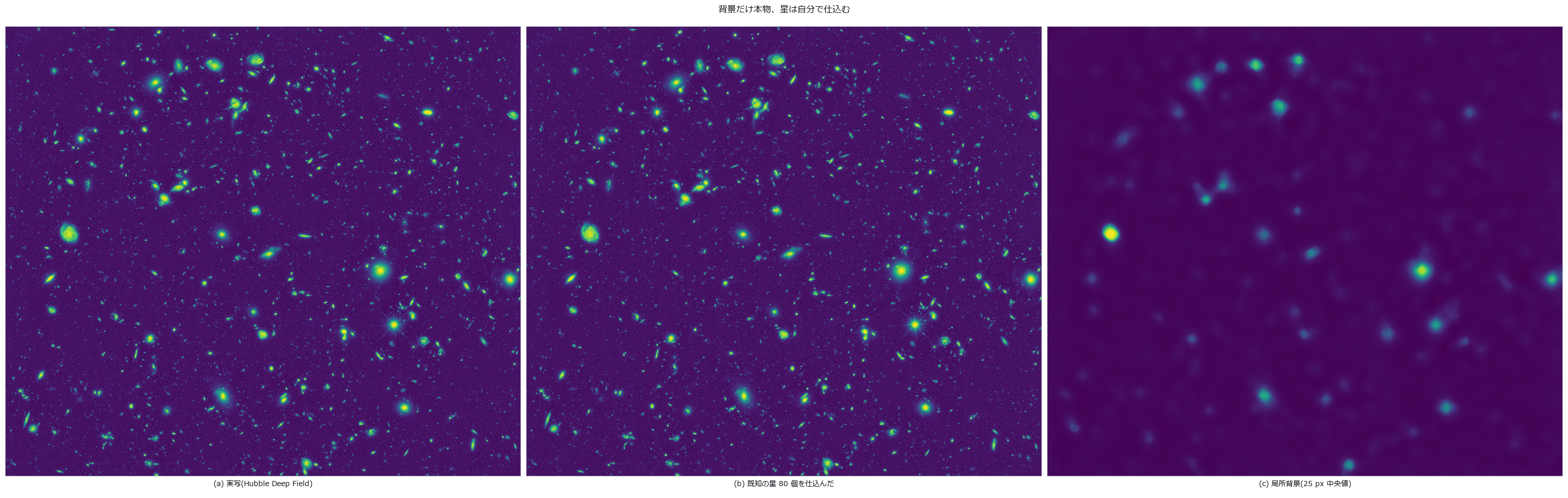
↑ Planting Known Stars in a Real Deep Field — Contamination Lies About the Measurement and the Confidence in the Same Direction ―― Gaussian stars of known flux planted in the real background of the Hubble Deep Field (NASA/STScI, public domain) — the truth is certain because it was planted, and only the background is real. The real sky is not Gaussian: a robust spread of 1,474 e- against a plain standard deviation of 6,698 e- (4.54x), so taking std for noise reports a detection limit 4.5 times too generous. The background is not one number either, ranging 3,176 to 8,448 e- across 195 tiles of 64x64, which leaves up to 3.6 sigma of systematic error after a single global subtraction. Even in the emptiest thirty per cent of the field a fixed amount leaks into the aperture: recovery runs 4.38x at F = 2,000 e- and 1.058x at 100,000, and it is an addition rather than a factor — 1 + C/(F·frac) fits all five points to within 0.9 %, with C = 6,677 e-, a mere 3.0 % of background times effective area. Predicting first that the bias falls below 10 % from 67,521 e- and then measuring there gives 1.086 against the predicted 1.100. In crowded positions the order of magnitude changes, 341x down to 7.80x: a median is robust to outliers, but when half the field is contaminated the median is the contamination. The confidence lies in the same direction — the op reports an SNR of 19.2 where the closed form on the same background gives 4.2 — so gating on S/N passes the contaminated measurements first.
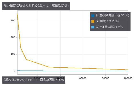
↑ The measurement ―― 開口 1 つあたり C = 6677 e- の足し算として説明できる。 (figure labels are in Japanese; the numbers are the same)
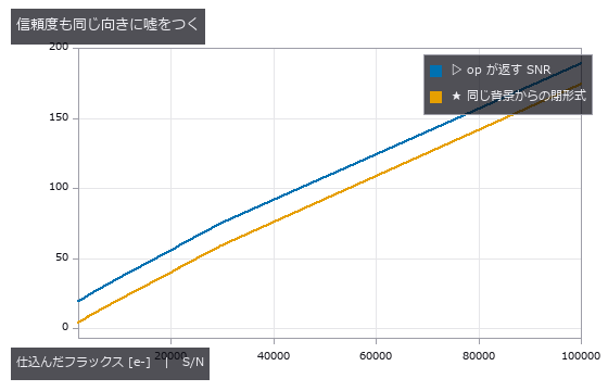
↑ SNR は測ったフラックスから作るので、混入で分子が膨らむと S/N も膨らむ(F=2000 で 19.2 対 4.2)。
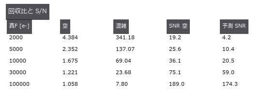
↑ 混雑側は桁が変わる。
py -3.11 examples/poc_real_sky_photometry.py
Source: examples/poc_real_sky_photometry.py
This run produced 4 figures in total - see them all
Ops used (notes): aperture_photometry
No.2026.080 —— River Surface Velocity — Separating a Discharge Proxy from Actual Discharge
An 8 m-wide synthetic river with 1.5 m/s peak is orthorectified to estimate u_s(y). Q_proxy=integral h(y)u_s(y)dy is a surface-velocity proxy; actual Q=integral h(y)alpha(y)u_s(y)dy requires separately measured depth and alpha(y) (literature mean about 0.8, condition-dependent). Velocity RMS is 0.074 m/s and proxy error -7.8%; -2.5 points of the -3.0% control come from bank trapezoidal integration. Removing the search limit leaves the dt cliff at k=4, consistent here with pair loss and within-window variation. Noise sigma=0.03 alone is below 0.001 m/s.
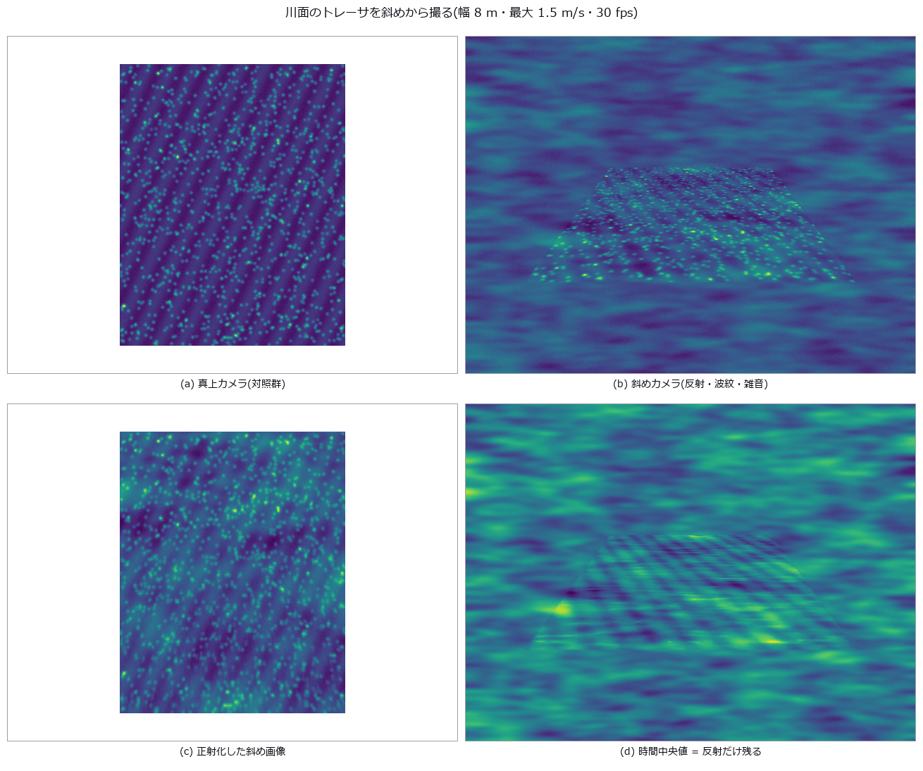
↑ River Surface Velocity — Separating a Discharge Proxy from Actual Discharge ―― An 8 m-wide synthetic river with 1.5 m/s peak is orthorectified to estimate u_s(y). Q_proxy=integral h(y)u_s(y)dy is a surface-velocity proxy; actual Q=integral h(y)alpha(y)u_s(y)dy requires separately measured depth and alpha(y) (literature mean about 0.8, condition-dependent). Velocity RMS is 0.074 m/s and proxy error -7.8%; -2.5 points of the -3.0% control come from bank trapezoidal integration. Removing the search limit leaves the dt cliff at k=4, consistent here with pair loss and within-window variation. Noise sigma=0.03 alone is below 0.001 m/s.
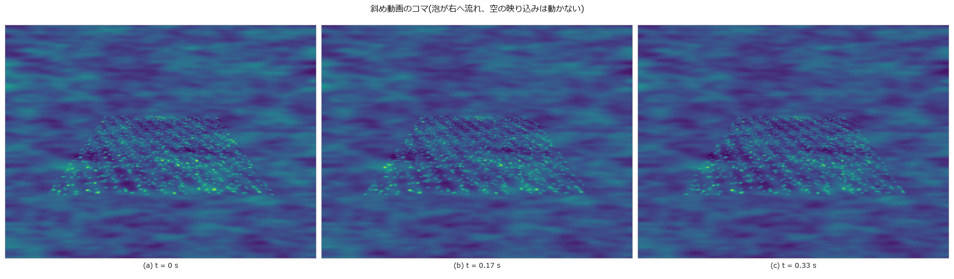
↑ The measurement (figure labels are in Japanese; the numbers are the same)
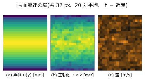
↑ この回の図
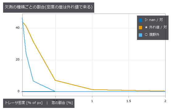
↑ この回の図
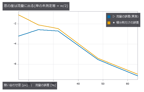
↑ この回の図
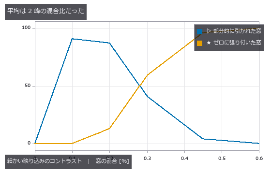
↑ この回の図
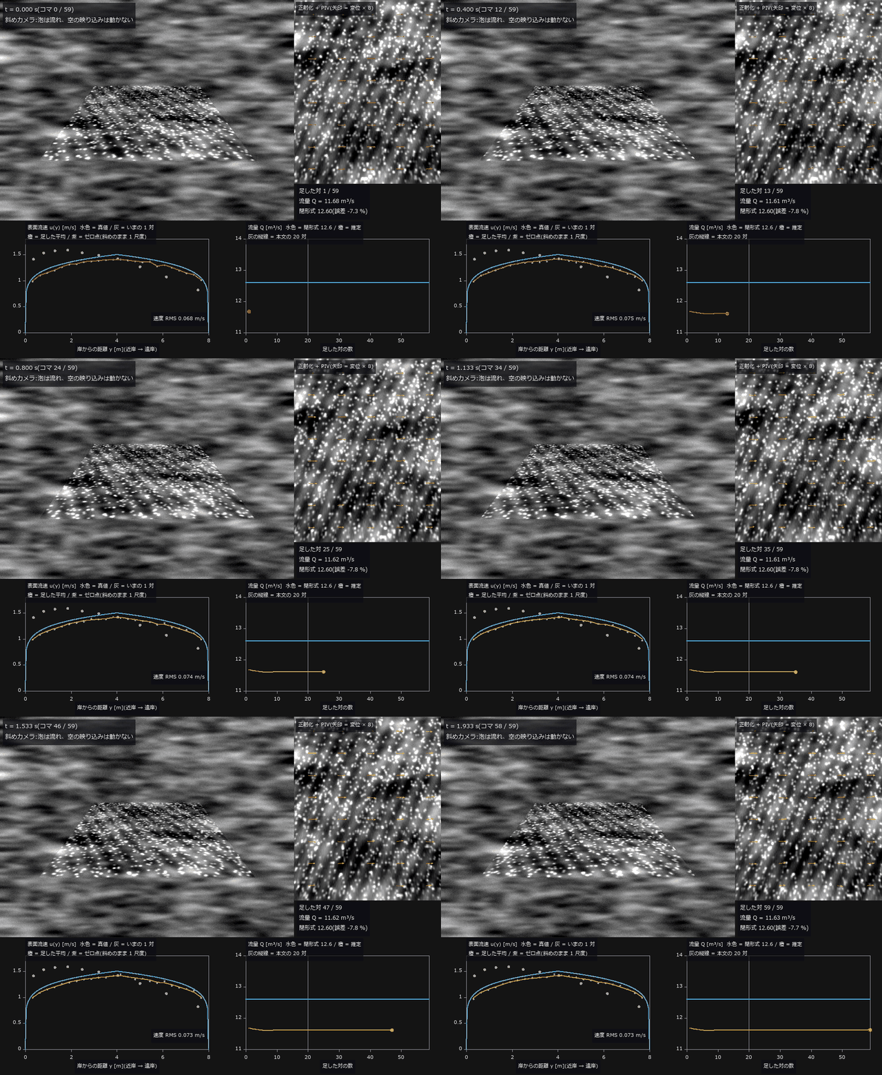
↑ The animation ―― 動画(60 コマ、30 fps で撮った 2 秒を 1/3 の速さで再生): 左上 = 斜めカメラ(泡が右へ流れ、空の映り込みは動かない)、右上 = 既知ホモグラフィで正射化したコマと、いま足した対の PIV 変位(矢印 × 8)。下段は対を 1 つずつ足した平均から出した表面流速 u(y)(橙)と流量 Q の推移。1 対だけで Q = 11.68 m³/s(-7.3 %)、本文と同じ 20 対で 11.62 m³/s(-7.8 %、閉形式 12.6)、59 対で 11.63 m³/s(-7.7 %)—— 対を足しても流量の誤差はほとんど動かない。平均で減るのは偶然誤差だけで、u(y) が真値より低めに出る偏りと岸 0 の台形則(だけで約 -2.5 %)は残る。紫は斜め画像のまま 1 尺度で直したゼロ点(近岸で速く遠岸で遅い)
py -3.11 examples/poc_river_surface_velocity.py
Source: examples/poc_river_surface_velocity.py
This run produced 13 figures in total - see them all
Ops used (notes): arrow · axes_frame · axes_transform · highpass_image · median · piv_cross_correlate · piv_ensemble_correlate · piv_error_stats · piv_outlier_mask · piv_replace_outliers · piv_sample_at_windows · piv_to_velocity · plot_series · sigma_clip_stack · text_box · ticks · warp_by_plane
No.2026.035 —— Sea-Ice Concentration — The Answer Depends on How Mixed Pixels Are Counted
Ice concentration from a PSF (point spread function)-blurred two-band ice/water image, by hard classification and by linear unmixing. Hard classification is off by -4.2 points, unmixing by +0.02. The bias is explained by the perimeter fraction (R² = 0.984) and crosses zero near a concentration of 0.49 — validate only there and it passes.
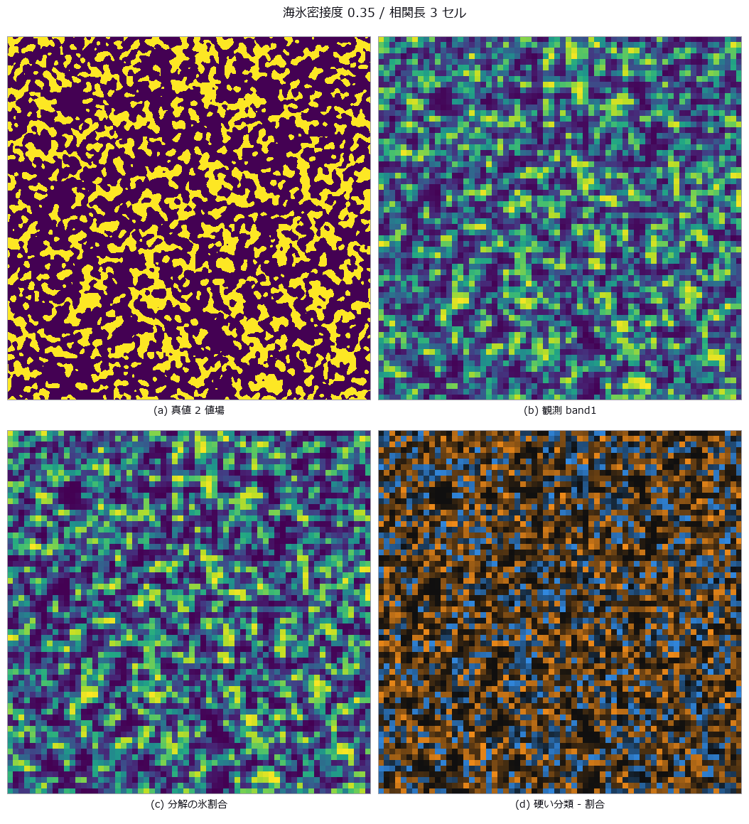
↑ Sea-Ice Concentration — The Answer Depends on How Mixed Pixels Are Counted ―― Ice concentration from a PSF (point spread function)-blurred two-band ice/water image, by hard classification and by linear unmixing. Hard classification is off by -4.2 points, unmixing by +0.02. The bias is explained by the perimeter fraction (R² = 0.984) and crosses zero near a concentration of 0.49 — validate only there and it passes.
Terms: PSF — The spatial response of an imaging system to a point object, describing how that point is blurred in the image.

↑ The measurement (figure labels are in Japanese; the numbers are the same)

↑ この回の図
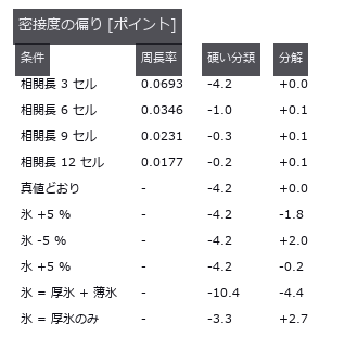
↑ 下 3 段は端成分 5 % 誤差と薄氷 20 %(2 端成分の分解)。
py -3.11 examples/poc_sea_ice_concentration.py
Source: examples/poc_sea_ice_concentration.py
This run produced 4 figures in total - see them all
Ops used (notes): blob_features · blob_label · gauss_filter · mat_lstsq
No.2026.110 —— Sweep Width — One Number Measured from Aerial Images Decides Whether the Search Works
Measure the lateral range curve p(x) from aerial imagery — detection probability as a function of cross-track distance — and hand its area, W = integral of p dx, to the search plan as the sweep width. This is where image processing and decision-making meet in a single number. The definition itself is demonstrated first: four curves of different shape (the measured p, a rectangle of width W, a triangle of base 2W, and a bimodal curve that cannot see nadir) all scaled to the same area of 256.2 m detect 0.2559 / 0.2563 / 0.2556 / 0.2566 of targets scattered uniformly over a half-width of 500 m, every one within 0.8 sigma of the predicted 0.2562. The shape vanishes; only the area survives. The cliff sits at coverage C = W v t / A = 1, printed in closed form before measuring: min(1, C) = 1.0000 and 1 - exp(-C) = 0.6321, against a rectangular control measuring 1.0000 and 0.6348 (the excess comes from having a finite 64 tracks; the exact value is 0.6350). Four predictions were wrong. Feeding the real p into a parallel sweep gives only 0.8464, not 1.000, because min(1, C) assumes the rectangular definite range law and a curve with tails overlaps its neighbouring tracks. The flatter curve was expected to be the more rectangle-like and therefore stronger, but it was the weaker (0.7705 against 0.8464): rectangle-like means standing inside W without tails, not being flat — while under random search the two curves tie, since random search only sees area. Ground resolution was expected to fall towards the swath edge, but for a nadir-looking central projection it is constant to 0.0e+00 relative spread; what falls is cos^4 vignetting, atmosphere and off-axis blur (an f-theta lens would coarsen the edge by 2.132 times). And subtracting a global background does nothing, because dividing by the whole-frame median and sigma is an affine map that cannot change the ranking (174.4 to 172.0 m); only a per-location subtraction helps (239.6 m). The optimum altitude lands in the interior at 220 m with W = 258.1 +/- 4.0 m, though 220 and 300 m are honestly not resolved apart; with an aircraft whose speed scales as min(1, h/600) the optimum moves to 420 m, so lowering the altitude to raise W does not work. The chaperone here is the false-alarm count, which concentrates at nadir rather than at the edge (113 in the 0-32 m band, zero in the outermost) because targets and whitecaps dim through the same cos^4: the best-seen place barks the most. Moving only the threshold slides W from 406 m to 170 m, so a sweep width quoted without a false-alarm rate says nothing at all.
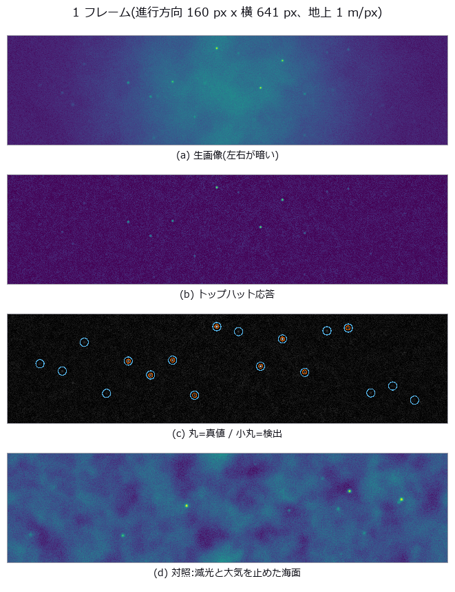
↑ Sweep Width — One Number Measured from Aerial Images Decides Whether the Search Works ―― Measure the lateral range curve p(x) from aerial imagery — detection probability as a function of cross-track distance — and hand its area, W = integral of p dx, to the search plan as the sweep width. This is where image processing and decision-making meet in a single number. The definition itself is demonstrated first: four curves of different shape (the measured p, a rectangle of width W, a triangle of base 2W, and a bimodal curve that cannot see nadir) all scaled to the same area of 256.2 m detect 0.2559 / 0.2563 / 0.2556 / 0.2566 of targets scattered uniformly over a half-width of 500 m, every one within 0.8 sigma of the predicted 0.2562. The shape vanishes; only the area survives. The cliff sits at coverage C = W v t / A = 1, printed in closed form before measuring: min(1, C) = 1.0000 and 1 - exp(-C) = 0.6321, against a rectangular control measuring 1.0000 and 0.6348 (the excess comes from having a finite 64 tracks; the exact value is 0.6350). Four predictions were wrong. Feeding the real p into a parallel sweep gives only 0.8464, not 1.000, because min(1, C) assumes the rectangular definite range law and a curve with tails overlaps its neighbouring tracks. The flatter curve was expected to be the more rectangle-like and therefore stronger, but it was the weaker (0.7705 against 0.8464): rectangle-like means standing inside W without tails, not being flat — while under random search the two curves tie, since random search only sees area. Ground resolution was expected to fall towards the swath edge, but for a nadir-looking central projection it is constant to 0.0e+00 relative spread; what falls is cos^4 vignetting, atmosphere and off-axis blur (an f-theta lens would coarsen the edge by 2.132 times). And subtracting a global background does nothing, because dividing by the whole-frame median and sigma is an affine map that cannot change the ranking (174.4 to 172.0 m); only a per-location subtraction helps (239.6 m). The optimum altitude lands in the interior at 220 m with W = 258.1 +/- 4.0 m, though 220 and 300 m are honestly not resolved apart; with an aircraft whose speed scales as min(1, h/600) the optimum moves to 420 m, so lowering the altitude to raise W does not work. The chaperone here is the false-alarm count, which concentrates at nadir rather than at the edge (113 in the 0-32 m band, zero in the outermost) because targets and whitecaps dim through the same cos^4: the best-seen place barks the most. Moving only the threshold slides W from 406 m to 170 m, so a sweep width quoted without a false-alarm rate says nothing at all.

↑ The measurement ―― 半幅 500 m に一様に撒いた 400000 個。予測 W/2X = 0.2562、モンテカルロの標準偏差 0.0007。 (figure labels are in Japanese; the numbers are the same)
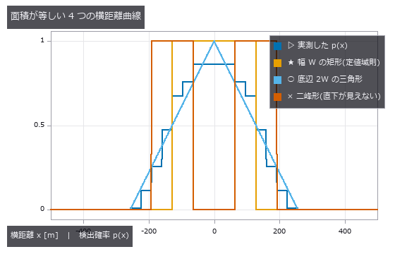
↑ 4 本とも面積 = W = 256 m。
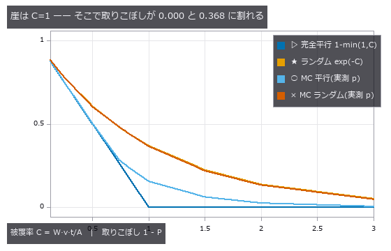
↑ 完全平行は C=1 でちょうど 0 に落ちるが、実測の横距離曲線では 0.154 残る(裾が隣の航跡と重なるため)。
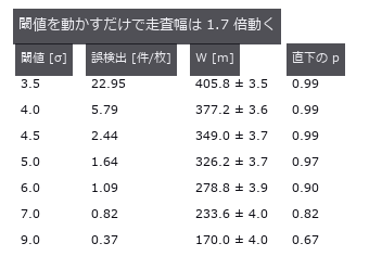
↑ だから走査幅は必ず誤検出率と対で報告する。

↑ 3 本とも誤検出 1.0 件/枚。
py -3.11 examples/poc_search_sweep_width.py
Source: examples/poc_search_sweep_width.py
This run produced 12 figures in total - see them all
Ops used (notes): gauss_filter · gray_tophat · integrate_funct_1d · laplace · ncc_locate · noise_sigma · photon_sample · relative_illumination · star_detect · tophat · vignette · xsk_blob_log
No.2026.036 —— Where Is the Edge of a Limb-Darkened Disc? The 50 % Rule Reads the Radius Small
A limb-darkened solar disc seen through seeing, its radius measured by the 50 % rule, by gradient maximum and by model fitting. The prediction ‘bias scales with the darkening coefficient’ failed: at u = 0.8 the bias is -12.76 px (pure geometry predicts -13.14 px). The cancellation point near threshold 0.26, where blur appears to have no effect, moves to 0.38 when u changes.
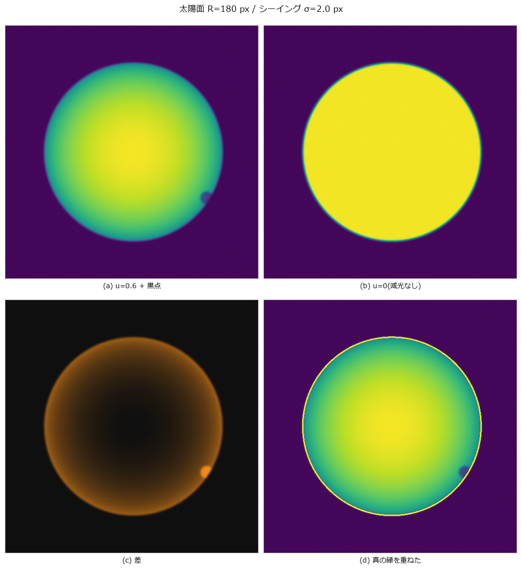
↑ Where Is the Edge of a Limb-Darkened Disc? The 50 % Rule Reads the Radius Small ―― A limb-darkened solar disc seen through seeing, its radius measured by the 50 % rule, by gradient maximum and by model fitting. The prediction ‘bias scales with the darkening coefficient’ failed: at u = 0.8 the bias is -12.76 px (pure geometry predicts -13.14 px). The cancellation point near threshold 0.26, where blur appears to have no effect, moves to 0.38 when u changes.

↑ The measurement (figure labels are in Japanese; the numbers are the same)
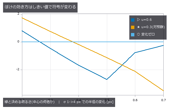
↑ この回の図
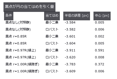
↑ 縁に載った黒点だけが効く(内側の黒点は縁の点列に入らない)。
py -3.11 examples/poc_solar_limb_darkening.py
Source: examples/poc_solar_limb_darkening.py
This run produced 4 figures in total - see them all
Ops used (notes): edge_points · gauss_filter · gaussian · gen_measure_rectangle2 · mat_lstsq · measure_pos
No.2026.037 —— To What Fraction of a Pixel Can a Star Be Located, and Where Is the Cliff?
Stars rendered from known celestial coordinates, located by four methods and compared with the Fisher-information bound. At S/N 298 the centroid (null) sits at 5.56x the bound and the background-subtracted centroid at 1.03x; no method beats the bound. At the faint end the null appears to beat it (0.2790 px versus 0.3471 px), but with a sensitivity of 0.038 it is merely returning the rounded initial guess.
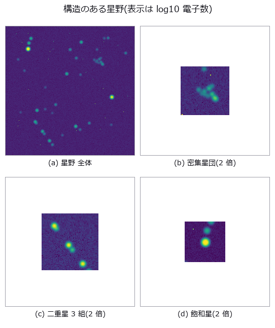
↑ To What Fraction of a Pixel Can a Star Be Located, and Where Is the Cliff? ―― Stars rendered from known celestial coordinates, located by four methods and compared with the Fisher-information bound. At S/N 298 the centroid (null) sits at 5.56x the bound and the background-subtracted centroid at 1.03x; no method beats the bound. At the faint end the null appears to beat it (0.2790 px versus 0.3471 px), but with a sensitivity of 0.038 it is merely returning the rounded initial guess.
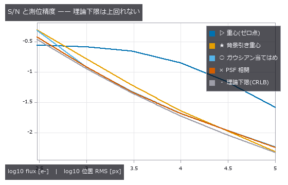
↑ The measurement ―― 暗い端で素の重心が下限を割って見えるのは「動かない推定器」だから(感度 0.038)。 (figure labels are in Japanese; the numbers are the same)
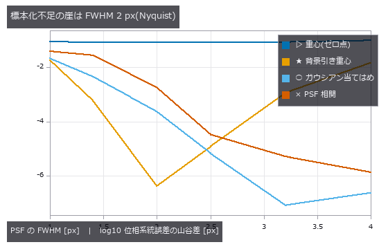
↑ 素の重心だけ FWHM に依らない(空の希釈)。
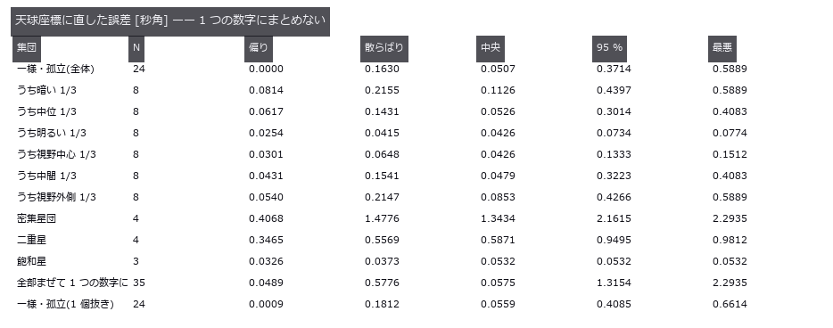
↑ 混ぜた中央値は孤立星とも二重星とも違う「どこでもない値」。
py -3.11 examples/poc_star_astrometry.py
Source: examples/poc_star_astrometry.py
This run produced 4 figures in total - see them all
Ops used (notes): gaussian · noise_sigma · psf_fit · star_detect · vector_to_similarity
No.2026.088 —— Counting tree rings and extracting the width series — ring count and width correlation fail separately
A 36-ring disc is synthesised in closed form with an off-centre pith, eccentric growth, circumferential wobble, wandering cracks, decay spots, grain texture and blur. A single-ray peak count (baseline) gets the ring count right in only 18 of 24 directions, yet the 6 wrong directions still give a width-series correlation of median 0.900. The consensus method (pith-centred polar unwrap, radius normalised by the disc edge, theta-median, 24 sector measure lines, median) returns exactly 36 rings, 0 missing, width correlation 0.996 (mean error 0.13 px). A 20 px pith error leaves the width correlation at 0.994: the cosine modulation lands on the radii (slope -14.9 px), not on the widths (-0.02 px); what it removes is the innermost rings (predicted 2 / measured 2). The thinnest ring is lost at 2.5 px (consensus) and 3.0 px (baseline), and at blur sigma 4 px the baseline counts 13 false rings.
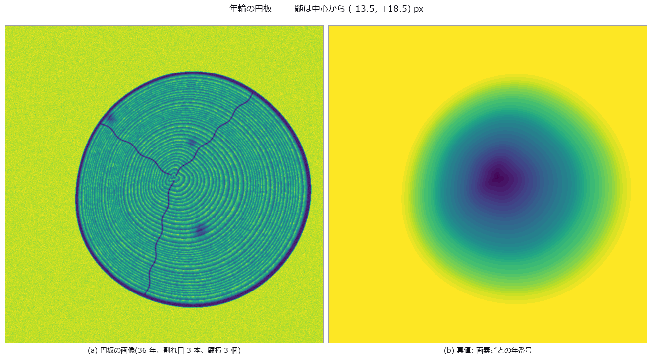
↑ Counting tree rings and extracting the width series — ring count and width correlation fail separately ―― A 36-ring disc is synthesised in closed form with an off-centre pith, eccentric growth, circumferential wobble, wandering cracks, decay spots, grain texture and blur. A single-ray peak count (baseline) gets the ring count right in only 18 of 24 directions, yet the 6 wrong directions still give a width-series correlation of median 0.900. The consensus method (pith-centred polar unwrap, radius normalised by the disc edge, theta-median, 24 sector measure lines, median) returns exactly 36 rings, 0 missing, width correlation 0.996 (mean error 0.13 px). A 20 px pith error leaves the width correlation at 0.994: the cosine modulation lands on the radii (slope -14.9 px), not on the widths (-0.02 px); what it removes is the innermost rings (predicted 2 / measured 2). The thinnest ring is lost at 2.5 px (consensus) and 3.0 px (baseline), and at blur sigma 4 px the baseline counts 13 false rings.

↑ The measurement ―― 偏心成長で境界が θ とともに斜めに走るので、正規化しないとθ 窓の中で外側の年輪がにじむ。 (figure labels are in Japanese; the numbers are the same)

↑ 展開図(横 = 半径 px、縦 = 角度)に、扇形ごとの測定線が拾った境界(赤、下)と真値(青、上)を重ねた。
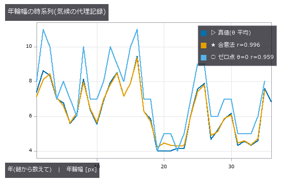
↑ ゼロ点は θ=0 方向の局所幅なので偏心成長ぶん尺度がずれる。

↑ 幅系列の相関はほぼ動かない。
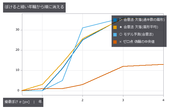
↑ この回の図
py -3.11 examples/poc_tree_ring_dendro.py
Source: examples/poc_tree_ring_dendro.py
This run produced 9 figures in total - see them all
Ops used (notes): derivate_funct_1d · find_peaks · gen_measure_rectangle2 · measure_pos · median_rect · polar_unwrap · smooth_funct_1d_gauss
No.2026.046 —— Counting Crop Green — Ground Truth as Per-Pixel Leaf Area Fraction
Cover fraction from a four-band field image, scored against the per-pixel leaf area fraction. The null (Otsu on the green channel) overshoots by +16.3 pp at mid-season, and since every method scatters by under 0.5 pp, nearly all of the difference is bias. At emergence on wet soil the null’s cover bias is -0.2 pp while precision and recall are both 0.000 — the number is right and not a single pixel is.
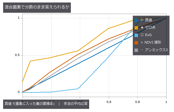
↑ Counting Crop Green — Ground Truth as Per-Pixel Leaf Area Fraction ―― Cover fraction from a four-band field image, scored against the per-pixel leaf area fraction. The null (Otsu on the green channel) overshoots by +16.3 pp at mid-season, and since every method scatters by under 0.5 pp, nearly all of the difference is bias. At emergence on wet soil the null’s cover bias is -0.2 pp while precision and recall are both 0.000 — the number is right and not a single pixel is.
Terms: Otsu — A histogram thresholding method that chooses the threshold maximizing the variance between the two resulting classes.
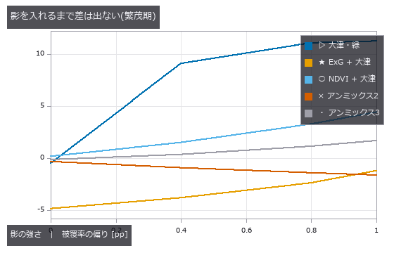
↑ The measurement ―― 影ゼロならゼロ点も悪くない。影は『暗さ』を手掛かりにする手法に直接刺さる。 (figure labels are in Japanese; the numbers are the same)
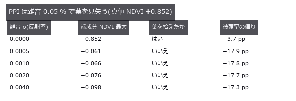
↑ 純粋な葉が 67 % ある場面。

↑ 白い画素の数だけが釣り合っている。
py -3.11 examples/poc_vegetation_cover.py
Source: examples/poc_vegetation_cover.py
This run produced 4 figures in total - see them all
Ops used (notes): cv_otsu · otsu · sk_otsu
No.2026.049 —— River Stage From an Oblique Photo — Ignoring Perspective Bends the Row-Number Error Into an Arc
The waterline detected on an obliquely photographed staff gauge and converted to stage. Linear conversion from two gauge marks bends off by up to -6.4 cm (at 1.00 m), and the sign is decided not by the stage but by whether the reading interpolates (-6.6 cm) or extrapolates (+16.3 cm). A four-point homography brings it under 0.2 cm; what remains is waterline detection, not perspective.
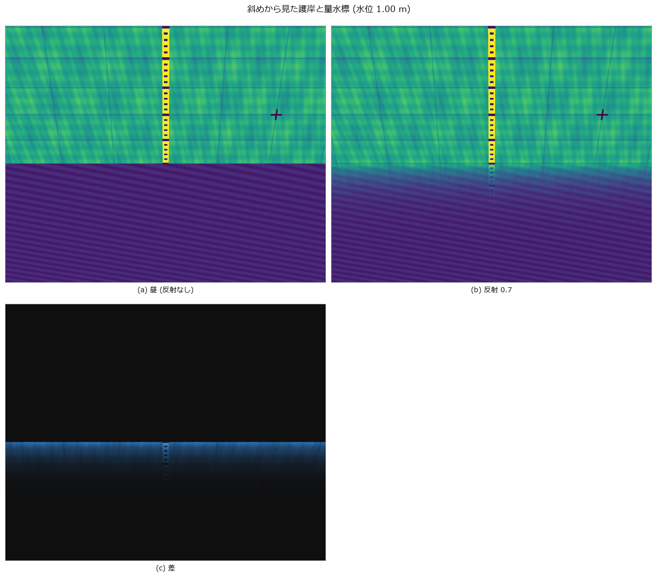
↑ River Stage From an Oblique Photo — Ignoring Perspective Bends the Row-Number Error Into an Arc ―― The waterline detected on an obliquely photographed staff gauge and converted to stage. Linear conversion from two gauge marks bends off by up to -6.4 cm (at 1.00 m), and the sign is decided not by the stage but by whether the reading interpolates (-6.6 cm) or extrapolates (+16.3 cm). A four-point homography brings it under 0.2 cm; what remains is waterline detection, not perspective.
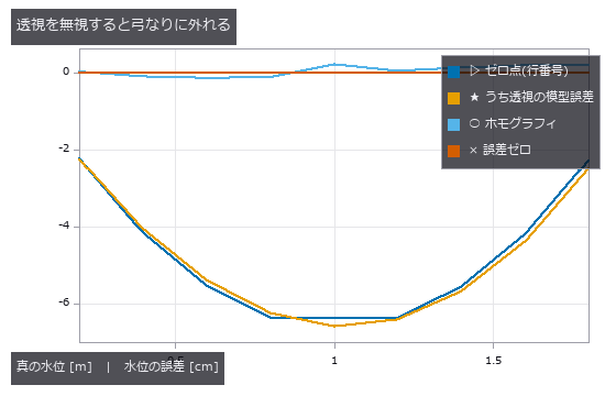
↑ The measurement (figure labels are in Japanese; the numbers are the same)
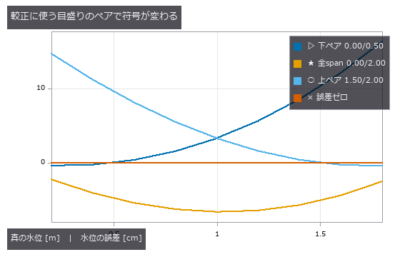
↑ この回の図
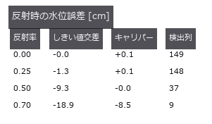
↑ 負 = 低く読む。
py -3.11 examples/poc_water_level.py
Source: examples/poc_water_level.py
This run produced 4 figures in total - see them all
Ops used (notes): gen_measure_rectangle2 · mat_svd · measure_pos · projective_trans_image · ransac_line · threshold
No.2026.217 —— Predicting Wheel Slip with Uncertainty on Real Martian Terrain and Planning a Path that Avoids the Slip Risk — Bekker / Wong–Reece and CVaR on a HiRISE DTM; outside the Data a Gaussian Process Calls a Stuck Slope ‘Slip 0.29’
On soft sand a wheel turns without the body advancing by the same amount (slip ratio s), and on steeper slopes the rover gets stuck. The existing terrain.traversability is purely geometric and has no notion of soil that cannot hold. With learning-free soil mechanics and light statistics: Bekker pressure–sinkage → numerical integration of Wong–Reece stresses on a rigid wheel → steady slip per slope angle → actual slip from a ground-facing camera’s translation and the wheel rotation → slip uncertainty (quantile regression with conformal calibration, and a Gaussian process) → a cost map of CVaR-discounted edge travel time and 8-neighbour Dijkstra. Closed form: traction at τ = 0 equals −Bekker’s compaction resistance to 1.9e-7. Dry sand (Mars gravity, 50 kg, 4 wheels) slips 0.219 at 20° and climbs at most 25.2°; the rigid-ground limit is 26.35° (a MuJoCo rigid wheel gives 25.83°, and does not match on sand). Visual-odometry slip error at most 0.0034. Coverage of the nominal 90 % band: quantile regression 0.915; the Gaussian process covers only 0.780 above 8°, is too wide on gentle slopes (0.992), and outside the data answers ‘slip 0.29’ at 32° (truth: stuck). On a HiRISE DTM (central peak of Balvicar crater, public domain, outside the repo via FULLSEYE_ROVERSLIP_DATA) the mean-shortest path is 672 m and the minimum-risk path 696 m, mean time +1.1 %, probability of getting stuck under true slip 2.23 % → 0.05 %. Traps: Bekker’s textbook sinkage factor (3 − n)/3 is 17 % too deep at n = 1.9; the 0.4.0 phase_correlation_fft (no window, full whitening) returned (1, 0) on a non-periodic crop of the ground (truth (−2, −5); its default was fixed on 2026-10-06). Honestly: the slip truth is synthetic, the soil type is unknown, and with one soil the two paths nearly coincide. 18 gates (15 on CI without data or mujoco, 3.1 s, curves at 5° and training data as observed); the figure run and –full use 1° curves and training data through visual odometry.

↑ Predicting Wheel Slip with Uncertainty on Real Martian Terrain and Planning a Path that Avoids the Slip Risk — Bekker / Wong–Reece and CVaR on a HiRISE DTM; outside the Data a Gaussian Process Calls a Stuck Slope ‘Slip 0.29’ ―― On soft sand a wheel turns without the body advancing by the same amount (slip ratio s), and on steeper slopes the rover gets stuck. The existing terrain.traversability is purely geometric and has no notion of soil that cannot hold. With learning-free soil mechanics and light statistics: Bekker pressure–sinkage → numerical integration of Wong–Reece stresses on a rigid wheel → steady slip per slope angle → actual slip from a ground-facing camera’s translation and the wheel rotation → slip uncertainty (quantile regression with conformal calibration, and a Gaussian process) → a cost map of CVaR-discounted edge travel time and 8-neighbour Dijkstra. Closed form: traction at τ = 0 equals −Bekker’s compaction resistance to 1.9e-7. Dry sand (Mars gravity, 50 kg, 4 wheels) slips 0.219 at 20° and climbs at most 25.2°; the rigid-ground limit is 26.35° (a MuJoCo rigid wheel gives 25.83°, and does not match on sand). Visual-odometry slip error at most 0.0034. Coverage of the nominal 90 % band: quantile regression 0.915; the Gaussian process covers only 0.780 above 8°, is too wide on gentle slopes (0.992), and outside the data answers ‘slip 0.29’ at 32° (truth: stuck). On a HiRISE DTM (central peak of Balvicar crater, public domain, outside the repo via FULLSEYE_ROVERSLIP_DATA) the mean-shortest path is 672 m and the minimum-risk path 696 m, mean time +1.1 %, probability of getting stuck under true slip 2.23 % → 0.05 %. Traps: Bekker’s textbook sinkage factor (3 − n)/3 is 17 % too deep at n = 1.9; the 0.4.0 phase_correlation_fft (no window, full whitening) returned (1, 0) on a non-periodic crop of the ground (truth (−2, −5); its default was fixed on 2026-10-06). Honestly: the slip truth is synthetic, the soil type is unknown, and with one soil the two paths nearly coincide. 18 gates (15 on CI without data or mujoco, 3.1 s, curves at 5° and training data as observed); the figure run and –full use 1° curves and training data through visual odometry.

↑ The measurement ―― real Mars terrain at 1:1 pixels: the mean-slip shortest path and the minimum slip-risk path (figure labels are in Japanese; the numbers are the same)

↑ the risk-aware path trims the peaks of the upper band at almost no extra length

↑ GP’s uniform noise is too wide on gentle slopes, too narrow on steep ones, and reverts to the mean past the data

↑ the slope a wheel can hold is where DP/W reaches sin(slope)

↑ no sinkage, no shear deformation: a rigid-contact simulator cannot show soft-soil slip
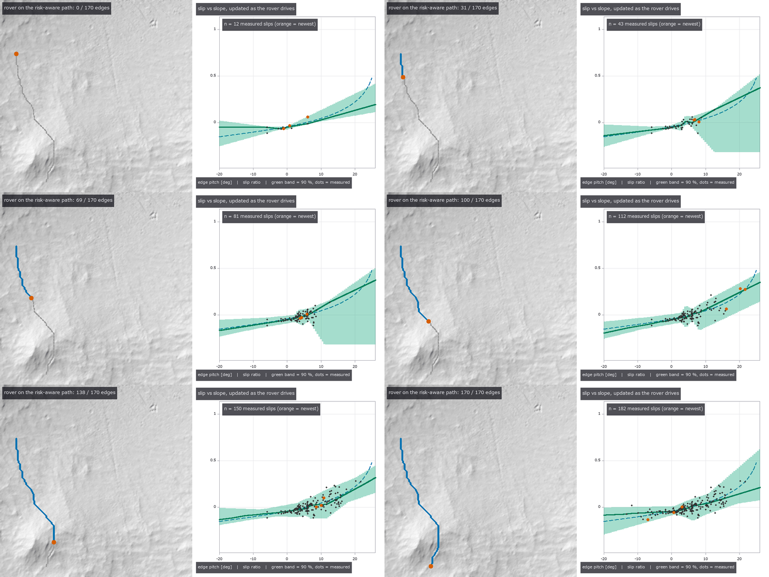
↑ The animation ―― as the rover drives, measured slips tighten the slip-vs-slope band (quantile regression, 90 %)
py -3.11 examples/poc_rover_slip_risk_path.py
Source: examples/poc_rover_slip_risk_path.py
This run produced 7 figures in total - see them all
Ops used (notes): bekker_wheel_sinkage · cvar_cost_map · fbm_height · fbm_params · ground_shift_track · odometry_slip · path_slip_risk · risk_aware_path · slip_gp_fit · slip_predict · slip_quantile_fit · slope_slip_curve · text_box · wheel_forces · wheel_sinkage · wheel_traction_curve
No.2026.136 —— There Are Two Kinds of Height, for Real — Putting a Height-Frame Mix-Up Under a Detector with 523 Published Survey Marks
| The synthetic companion (poc_geodetic_height_frames) showed that mixing ellipsoidal and orthometric heights costs tens of metres, using numbers we made ourselves. This exhibit checks the same claim against numbers somebody else measured and published. An NGS datasheet gives, for one mark, the ellipsoidal height h (NAD 83(2011)), the orthometric height H (NAVD 88), the geoid height N (GEOID18) and the Cartesian coordinates (x,y,z) — all four — so 523 marks were taken from the Colorado Front Range, where the geoid is steep enough for interpolation error to show. An existing operator was finally checked against the outside world: dem_geodetic_to_ecef lands within 0.5 mm rms (0.8 mm worst) of the published Cartesian coordinates, and the inverse closes to 7.1e-09 degrees, inside the 9.0e-09-degree floor set by the millimetre rounding of the published data — until now this operator had only been checked against its own inverse, which tests consistency, not correctness. Interpolating a coarse grid costs more than a generation of geoid model: bilinear interpolation of a 0.25-degree GEOID18 grid differs from the published point values by 11.1 cm rms (44.5 cm worst), while GEOID18 minus GEOID12B is -1.0 cm on average (range -9.8 to +6.3 cm). Fifteen of the 523 marks fall outside the grid and are refused rather than clamped, because an extrapolated undulation is not a survey value. A height-frame mix-up does not look like an outlier: putting h into the orthometric column places every single mark exactly on the line -N, lifting the whole table by 16.75 m. And the residual sorts the marks by how they were surveyed even though it never reads that metadata: median | h-H-N | is 1.6 cm for levelling, 1.9 cm for network adjustment, 3.8 cm for GPS observation and 8.3 cm (1.02 m worst) for VERTCON3, a modelled datum conversion. Even the published triples do not close exactly (10.6 cm rms): NAVD 88 comes from levelling and GEOID18 from gravity, and the mismatch shows up here. Only a 56 KB aggregate ships; the raw download stays out of the repository. |
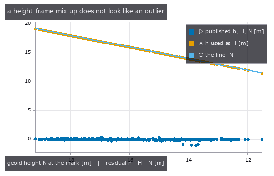
| *↑ There Are Two Kinds of Height, for Real — Putting a Height-Frame Mix-Up Under a Detector with 523 Published Survey Marks ―― The synthetic companion (poc_geodetic_height_frames) showed that mixing ellipsoidal and orthometric heights costs tens of metres, using numbers we made ourselves. This exhibit checks the same claim against numbers somebody else measured and published. An NGS datasheet gives, for one mark, the ellipsoidal height h (NAD 83(2011)), the orthometric height H (NAVD 88), the geoid height N (GEOID18) and the Cartesian coordinates (x,y,z) — all four — so 523 marks were taken from the Colorado Front Range, where the geoid is steep enough for interpolation error to show. An existing operator was finally checked against the outside world: dem_geodetic_to_ecef lands within 0.5 mm rms (0.8 mm worst) of the published Cartesian coordinates, and the inverse closes to 7.1e-09 degrees, inside the 9.0e-09-degree floor set by the millimetre rounding of the published data — until now this operator had only been checked against its own inverse, which tests consistency, not correctness. Interpolating a coarse grid costs more than a generation of geoid model: bilinear interpolation of a 0.25-degree GEOID18 grid differs from the published point values by 11.1 cm rms (44.5 cm worst), while GEOID18 minus GEOID12B is -1.0 cm on average (range -9.8 to +6.3 cm). Fifteen of the 523 marks fall outside the grid and are refused rather than clamped, because an extrapolated undulation is not a survey value. A height-frame mix-up does not look like an outlier: putting h into the orthometric column places every single mark exactly on the line -N, lifting the whole table by 16.75 m. And the residual sorts the marks by how they were surveyed even though it never reads that metadata: median | h-H-N | is 1.6 cm for levelling, 1.9 cm for network adjustment, 3.8 cm for GPS observation and 8.3 cm (1.02 m worst) for VERTCON3, a modelled datum conversion. Even the published triples do not close exactly (10.6 cm rms): NAVD 88 comes from levelling and GEOID18 from gravity, and the mismatch shows up here. Only a 56 KB aggregate ships; the raw download stays out of the repository.* |

↑ The measurement ―― 523 NGS marks, each publishing ellipsoidal height h (NAD 83), orthometric height H (NAVD 88) and geoid height N (GEOID18). The residual h - H - N is not exactly zero: NAVD 88 and GEOID18 were built from different measurements, and the mismatch shows up here at the centimetre level (rms 0.106 m, median -0.004 m). 74 of 523 marks exceed 0.1 m (figure labels are in Japanese; the numbers are the same)
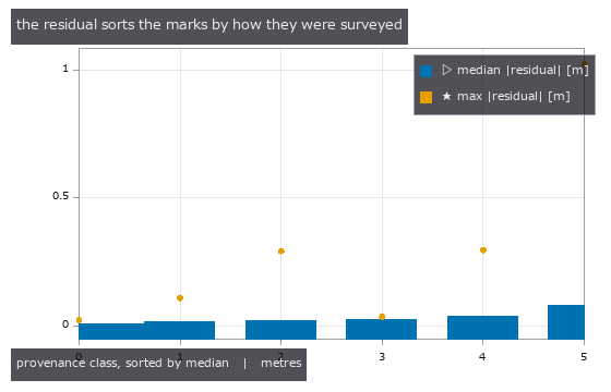
↑ dem_height_frame_residual reads only the three height columns — never the metadata saying how each mark was measured.

↑ the published GEOID18 undulation on a 0.25-degree grid over the Colorado Front Range (-19.40 to -11.15 m, 9x7 nodes).

↑ GEOID18 minus GEOID12B on the same nodes: mean -0.010 m, range -0.098 to +0.063 m.
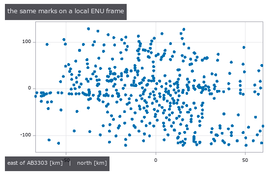
↑ 523 marks placed in the east-north-up frame of one of them (AB3303).
py -3.11 examples/poc_geodetic_benchmarks_real.py
Source: examples/poc_geodetic_benchmarks_real.py
This run produced 9 figures in total - see them all
Ops used (notes): dem_datum_shift_3param · dem_ecef_to_geodetic · dem_enu_from_geodetic · dem_geodetic_from_enu · dem_geodetic_to_ecef · dem_geoid_height · dem_height_frame_convert · dem_height_frame_residual
No.2026.147 —— Scoring Gravitational-Lens Images with Ordinary Industrial Measurement Operators
| Gravitational lensing carries exact invariants that can be measured straight off the picture, and the tools that measure them are ordinary 2-D operators already in the box: connected components, area and centroid. Writing a point-mass lens in units of the Einstein radius, a source at position u produces images at theta = (u +/- sqrt(u^2+4))/2 with magnifications mu = (u^2+2)/(2 u sqrt(u^2+4)) +/- 1/2, from which two equalities hold no matter where the source sits: the product of the image positions is exactly -1, and the difference of the magnifications is exactly 1, an integer. Across nine source positions the first moves by 8.9e-16 and the second by 2.2e-16. The first core finding is that the integer comes out of the picture: rendering by tracing image-plane pixels back to the source plane, splitting the result into two images with blob_label and subtracting their areas gives a deviation from 1 of 0.0660, 0.0216 and 0.0126 on grids of 801, 1601 and 3201 - measured from the drawing, not read off the model. The second is that surface brightness is exactly conserved, as Liouville’s theorem requires: the interior value of the images stays at 1.000000000000000 while the area falls from 2,322 to 480 pixels, so one frame yields both a quantity that does not change and one that does. The third is that the width of the Einstein ring equals the radius of the source, because the radial magnification on the ring is exactly one half; across four source radii the largest discrepancy is 7.2e-05. The fourth is that the singularity manufactures a one-pixel false image: with the source exactly behind the lens the image should be a single ring, yet the connected components number two, the extra one being the pixel at the lens centre where the deflection diverges - a gate that counts images lies here. Two predictions were wrong and have been left in. The first was that measuring from the picture would struggle where the faint image shrinks, at u = 1.5; in fact the worst case at every resolution was u = 0.3, near the caustic, and the faint image at u = 1.5 still covers 209 pixels - the difficulty is not small images but images stretched into thin arcs. The second was the anti-aliasing itself: the edge coverage was being computed from a distance in the source plane while the pixel width belongs to the image plane, and dividing the distance field by its image-plane gradient dropped the u = 0.3 deviation from 0.0214 to 0.0126. For a singular isothermal sphere the image separation is independent of source position at twice the Einstein radius, with a largest discrepancy of 9.3e-03 over four positions. In the animation of a source crossing behind the lens, the measured magnification tracks the closed form to a relative difference of 0.009 while | u | >= 0.3 and opens to 0.161 closer to the caustic, so the range over which the method works is reported alongside the claim. The figures use a calibration target as the source - four concentric rings and twelve radial spokes - so the shear can be read by eye. No new operator was added. |

| *↑ Scoring Gravitational-Lens Images with Ordinary Industrial Measurement Operators ―― Gravitational lensing carries exact invariants that can be measured straight off the picture, and the tools that measure them are ordinary 2-D operators already in the box: connected components, area and centroid. Writing a point-mass lens in units of the Einstein radius, a source at position u produces images at theta = (u +/- sqrt(u^2+4))/2 with magnifications mu = (u^2+2)/(2 u sqrt(u^2+4)) +/- 1/2, from which two equalities hold no matter where the source sits: the product of the image positions is exactly -1, and the difference of the magnifications is exactly 1, an integer. Across nine source positions the first moves by 8.9e-16 and the second by 2.2e-16. The first core finding is that the integer comes out of the picture: rendering by tracing image-plane pixels back to the source plane, splitting the result into two images with blob_label and subtracting their areas gives a deviation from 1 of 0.0660, 0.0216 and 0.0126 on grids of 801, 1601 and 3201 - measured from the drawing, not read off the model. The second is that surface brightness is exactly conserved, as Liouville’s theorem requires: the interior value of the images stays at 1.000000000000000 while the area falls from 2,322 to 480 pixels, so one frame yields both a quantity that does not change and one that does. The third is that the width of the Einstein ring equals the radius of the source, because the radial magnification on the ring is exactly one half; across four source radii the largest discrepancy is 7.2e-05. The fourth is that the singularity manufactures a one-pixel false image: with the source exactly behind the lens the image should be a single ring, yet the connected components number two, the extra one being the pixel at the lens centre where the deflection diverges - a gate that counts images lies here. Two predictions were wrong and have been left in. The first was that measuring from the picture would struggle where the faint image shrinks, at u = 1.5; in fact the worst case at every resolution was u = 0.3, near the caustic, and the faint image at u = 1.5 still covers 209 pixels - the difficulty is not small images but images stretched into thin arcs. The second was the anti-aliasing itself: the edge coverage was being computed from a distance in the source plane while the pixel width belongs to the image plane, and dividing the distance field by its image-plane gradient dropped the u = 0.3 deviation from 0.0214 to 0.0126. For a singular isothermal sphere the image separation is independent of source position at twice the Einstein radius, with a largest discrepancy of 9.3e-03 over four positions. In the animation of a source crossing behind the lens, the measured magnification tracks the closed form to a relative difference of 0.009 while | u | >= 0.3 and opens to 0.161 closer to the caustic, so the range over which the method works is reported alongside the claim. The figures use a calibration target as the source - four concentric rings and twelve radial spokes - so the shear can be read by eye. No new operator was added.* |
| [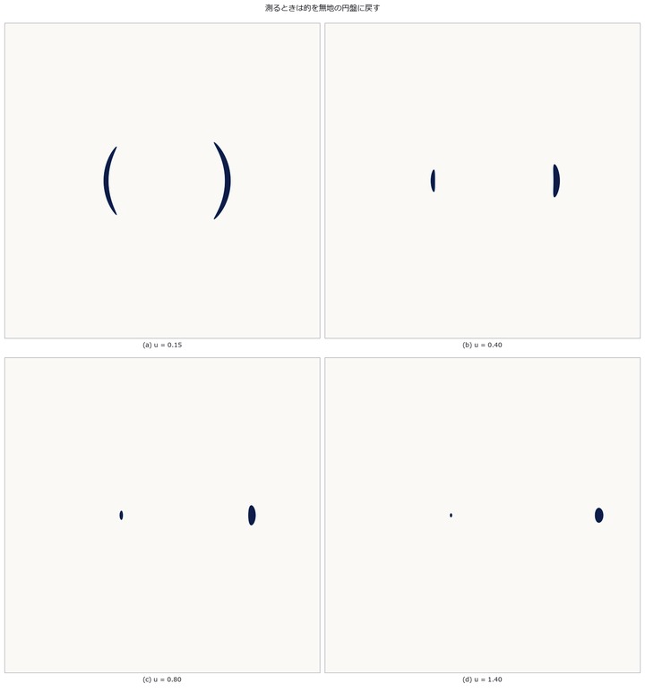](https://raw.githubusercontent.com/furuse-kazufumi/fullseye/master/docs/articles/assets/poc/poc_gravitational_lens_invariants/02_disc_images_vs_u.png) |
| *↑ The measurement ―― 面積を測るのに模様は要らない。明るいほうの像は外側(θ₊ > 1)、暗いほうは内側( | θ₋ | < 1)に出て、離れるほど内側の像は小さく暗くなる。 (figure labels are in Japanese; the numbers are the same)* |

↑ 9 通りの u で θ₊·θ₋ は −1 から 8.9e-16、μ₊ − μ₋ は 1 から 2.2e-16 しか動かない。

↑ 像の内部の値はどちらも厳密に 1.000000000000000。
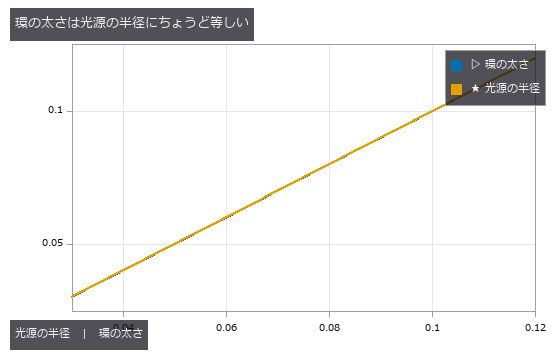
↑ 環の上では動径方向の倍率が厳密に 1/2 なので、直径 2ρ の光源は太さ ρ の環になる。
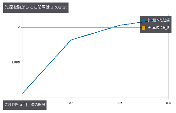
↑ 重心は blob_label で分けた成分ごとに、被覆率で重みを付けて出している。
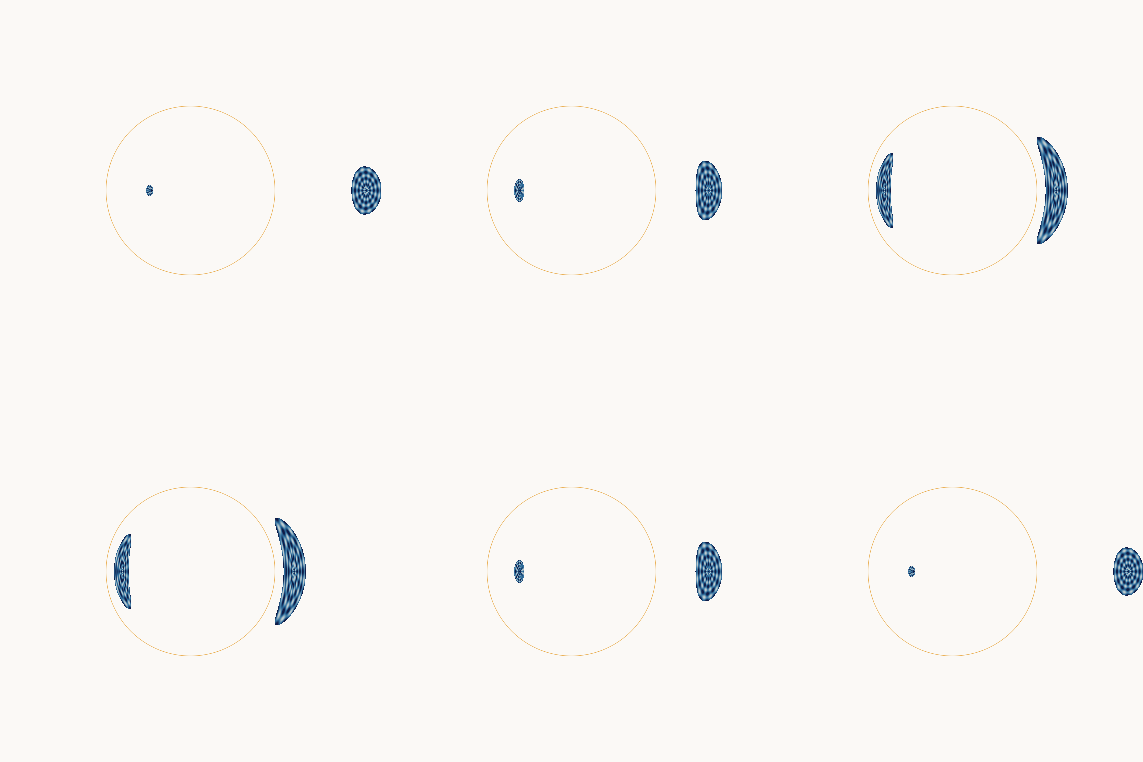
↑ The animation ―― 光源がレンズの裏を横切る(図は校正ターゲット)。最接近で 2 つの像が伸びて環に近づく。倍率の数字は同じ光源位置を無地の円盤で描き直して測ったもので、最大 19.61 倍。
py -3.11 examples/poc_gravitational_lens_invariants.py
Source: examples/poc_gravitational_lens_invariants.py
This run produced 12 figures in total - see them all
Ops used (notes): blob_label
No.2026.257 —— Weedy-Rice Cover — Supervised Linear Discrimination without Deep Learning
UAV paddy RGB is divided into 16 px blocks. A supervised ten-feature Fisher LDA is fitted on train, the grid candidate selected on validation, and 148 test images scored once. Predeclared edges are 5/25/50%. Agreement is 0.574 (majority 0.345), kappa 0.424, cover correlation 0.826 and IoU 0.397 (random 0.189). Swapping R/G gives kappa -0.023. Holding out flight dates, one different-season date has within-date correlation 0.14; the bundled split measures other frames from seen flights.
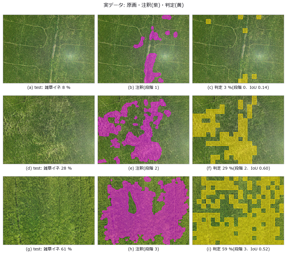
↑ Weedy-Rice Cover — Supervised Linear Discrimination without Deep Learning ―― UAV paddy RGB is divided into 16 px blocks. A supervised ten-feature Fisher LDA is fitted on train, the grid candidate selected on validation, and 148 test images scored once. Predeclared edges are 5/25/50%. Agreement is 0.574 (majority 0.345), kappa 0.424, cover correlation 0.826 and IoU 0.397 (random 0.189). Swapping R/G gives kappa -0.023. Holding out flight dates, one different-season date has within-date correlation 0.14; the bundled split measures other frames from seen flights.
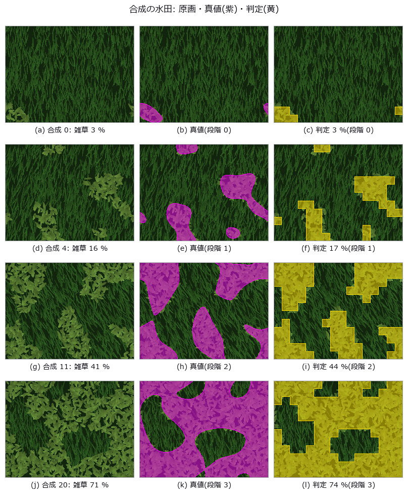
↑ The measurement ―― 作物は細く濃い葉が畝の向きに揃い、雑草は広く明るい葉がばらばらの向き。雑草の割合は乱数場の分位点で厳密に置いた。判定は 16 px 角の区画ごとの Fisher 判別。 (figure labels are in Japanese; the numbers are the same)

↑ 葉の形と配置は同じ乱数で同じ。

↑ データ付属の分割は同じ飛行の隣り合うコマを train と test に分ける(コマは重なる)。
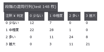
↑ 対角が一致。
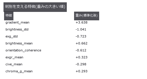
↑ 正の重みは雑草イネの側。
py -3.11 examples/poc_weed_rice_ratio.py
Source: examples/poc_weed_rice_ratio.py
This run produced 10 figures in total - see them all
Ops used (notes): cover_ratio_grade · fisher_lda_fit · fisher_lda_score · msa_attribute_agreement · plant_color_index · snic_superpixels · superpixel_color_texture_features
This museum was built together with Claude Code. I set the questions and the direction; Claude Code did the implementation, the sweeps, the control groups and the adversarial checks. That division of labour is what made it possible to run 53 PoCs and collect their figures in two days. If you want to try it, this invitation link gives you a one-week free trial: claude.ai/referral/0sqPw8E_lw
If even one exhibit was worth your time, a like or a stock helps: the reactions decide which wing grows next, so tell me in the comments which measurement from your own field you would want to see. And if you swapped in real data and the cliff moved, that is the story I most want to hear.