fullseye
The Industrial Inspection Wing — A Passing Number and a Failing Number Can Coexist
Numbers on an inspection line decide pass or fail, so there is a strong pull toward collapsing them into a single figure. The ten exhibits in this room show what disappears the moment you do: a pooled ROC that hides one defect class’s blind spot in woven fabric, veiling glare that leaves the MTF passing while the black level fails, a barcode decoder that looks better by read rate alone because it never says ‘unreadable’.
Every ground truth is planted: a closed-form periodic background, the laser-profile h(x), the analytic 1-D heat-conduction solution, closed-form bearing defect frequencies. That is what lets each exhibit measure ‘where detection stops working’ instead of ‘detection worked’, without fitting the threshold afterwards.
The other shared feature is that failure arrives as a cliff, not a slope: 15 versus 16 degrees of tilt, a 25-second versus a 4-second fitting window, ΔT of 1.6 K. Most of those positions can be predicted from geometry or physics first, and wherever they could be, the prediction is checked against the measurement.
1. Where a 1-D Barcode Stops Reading — Counting Misreads and Unreadables Separately
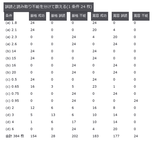
↑ Where a 1-D Barcode Stops Reading — Counting Misreads and Unreadables Separately ―― A home-made simple code (not a real standard) damaged four ways, with success, misread and unreadable counted as three separate outcomes. Over the 384 images past the onset of damage, the strict decoder that checks run structure misreads 7.3 %, while the lenient decoder that always returns nine digits misreads 46.1 % — and has the higher success rate (47.7 % versus 40.1 %). The tilt cliff is pure geometry (predicted 15.95 degrees) and lands between 15 and 16 degrees.
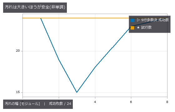
↑ The measurement ―― 小さい汚れは行が「読めてしまう」ので誤った票を投じる。大きい汚れは棄権するので多数決が効く。 (figure labels are in Japanese; the numbers are the same)
py -3.11 examples/poc_barcode_1d.py
Source: examples/poc_barcode_1d.py
Ops used (notes): decode_barcode · gen_measure_rectangle2 · measure_pos · vol_edge_probe
2. Electrode tortuosity from CT — the rule of thumb only sees porosity
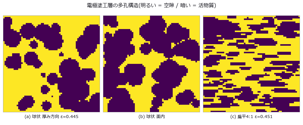
↑ Electrode tortuosity from CT — the rule of thumb only sees porosity ―― A synthetic micro-CT of a lithium-ion electrode coating, measured for porosity and tortuosity. Against the shop-floor default (Bruggeman tau = eps^-0.5) we put the real thing: the steady-state diffusion equation solved on the same volume. At eps = 0.4448 the rule gives 1.499 against a true 1.843 (-18.6 %), and sweeping eps from 0.691 to 0.168 widens the error from -8.2 % to -69.1 % (fitted exponents 1.78 and 2.70 — never 1.5). The geodesic tortuosity that imaging papers report (1.182) merely has a square that hugs Bruggeman to within 1 %; neither goes near the truth. The decisive control: hold porosity at 0.4448 vs 0.4510 and flatten the particles 4:1, and through-plane tau jumps 1.843 -> 6.794 (anisotropy 0.97 -> 4.20) while the rule returns the same 1.5 for both — in-plane looks right (-8 %), through-plane collapses (-78 %). Closed pores peak at 1.92 % and are not the culprit; the necks, 0.40 of a particle radius wide, are. We predicted a resolution cliff and found none: coarsening the voxel 5.5x moves eps by -0.4 % but tau by +72 %, with no warning of any kind.

↑ The measurement ―― 左: 上端 1 / 下端 0 の濃度場。等濃度線が固相を避けて曲がる分が遠回り。右: bond ごとの散逸(明るいほど流れが集中している = 首)。 (figure labels are in Japanese; the numbers are the same)
py -3.11 examples/poc_battery_electrode_tortuosity.py
Source: examples/poc_battery_electrode_tortuosity.py
Ops used (notes): vol_distance_transform · vol_label
3. Rolling-Bearing Diagnosis — How Deep in Noise Can It Still Be Caught?
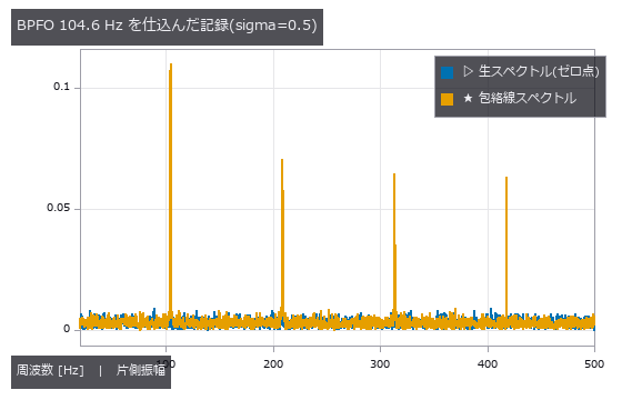
↑ Rolling-Bearing Diagnosis — How Deep in Noise Can It Still Be Caught? ―― An impulse train synthesised at the closed-form defect frequency (BPFO 104.556 Hz), sunk into noise, with detection rates of the raw spectrum and the envelope spectrum side by side. The worst SNR at which 10 of 10 seeds still detect is -0.9 dB for the raw spectrum and -18.4 dB for the envelope, a 17.5 dB gap. But a record with no defect at all still produces a global prominence of 43; had the threshold not been set from the null recording, this PoC would have been its own false positive.
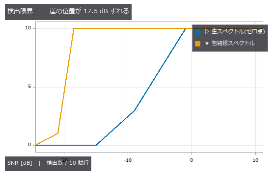
↑ The measurement ―― どちらも最悪条件では 0 に落ちる。包絡線は万能ではなく、崖が悪い SNR 側へ動くだけ。 (figure labels are in Japanese; the numbers are the same)
py -3.11 examples/poc_bearing_diagnosis.py
Source: examples/poc_bearing_diagnosis.py
Ops used (notes): bearing_defect_frequencies · envelope_spectrum · spectral_kurtosis · spectrum · synthesize_bearing_signal
4. Bump coplanarity versus substrate warpage — subtract too much and the real defect goes with it
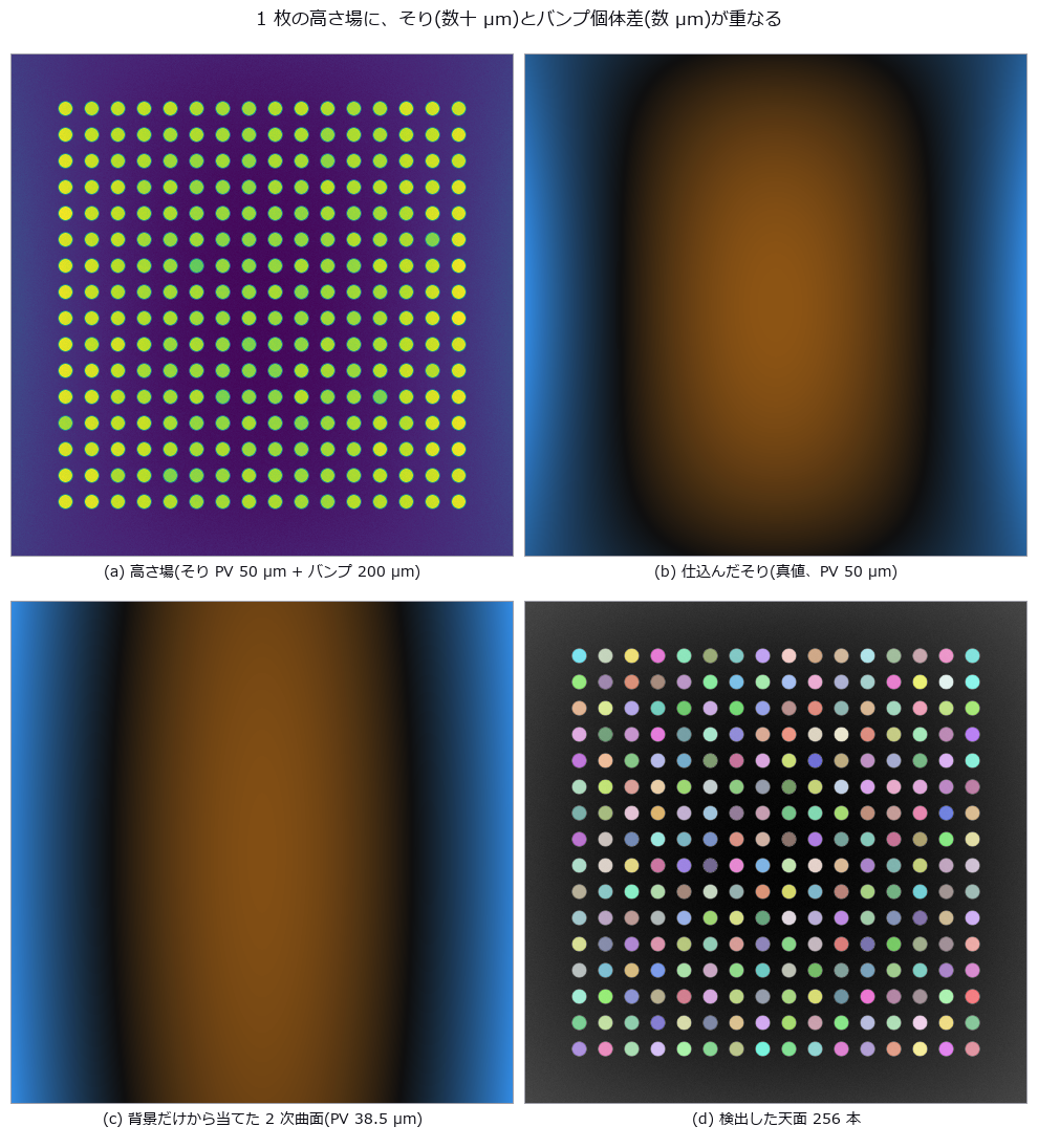
↑ Bump coplanarity versus substrate warpage — subtract too much and the real defect goes with it ―― A height map of 256 Cu pillars is planted with 50 µm PV warpage, 4 µm 1-sigma pillar-to-pillar spread and six short bumps. The zero point — subtract only a least-squares plane, the JEDEC seating plane — reads the individual deviation with 8.84 µm RMS error (2.2x the real spread), raising 58 false rejects while missing one genuinely short bump. A quadratic reference surface brings it to 1.23 µm with zero false rejects; a cubic one is worse (1.37 µm), because the planted high-order mode is quartic and the four extra terms only absorb real signal. The cliff is predictable from geometry: the quadratic fit degrades to the 4 µm level at 169.9 µm PV (predicted) versus 169.4 µm (measured). Adding a real low-order defect — the centre sagging 8 µm — removes 88.2 % of it from the residual while the short-bump detection count stays at 5 of 6, and misses rise from 0 to 2; the lost signal reappears as warpage growing 30.06 to 36.20 µm.
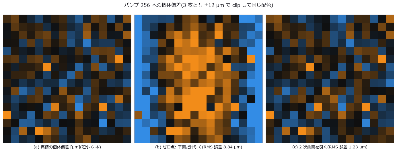
↑ The measurement (figure labels are in Japanese; the numbers are the same)
py -3.11 examples/poc_bump_coplanarity.py
Source: examples/poc_bump_coplanarity.py
Ops used (notes): auto_threshold · background_flatten · blob_features · blob_label · blob_overlay · eval_poly_surface · fit_poly_surface · surface_form_error
5. Concrete Crack Width Is Thinner Than a Pixel — Counting Width Versus Integrating Width
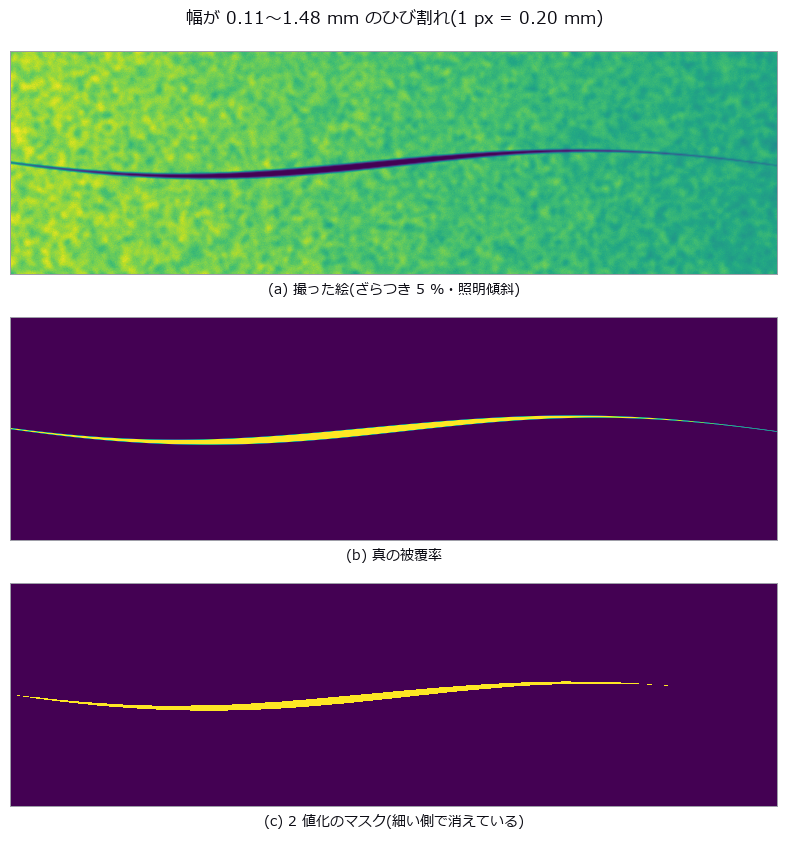
↑ Concrete Crack Width Is Thinner Than a Pixel — Counting Width Versus Integrating Width ―― Cracks from 0.05 to 2.0 mm wide in a field where 1 px = 0.20 mm, measured by thresholding-and-counting and by integrating the intensity deficit across the crack. Thresholding returns nothing at or below 0.20 mm and reports 0.200 mm for all four true widths between 0.25 and 0.40 mm. Integration tracks continuously down to 0.05 mm (0.25 px), but curved illumination adds a +0.1741 mm offset under a first-order baseline (+0.0062 mm with second order).
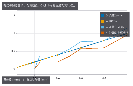
↑ The measurement ―― 2 値化の 2 本は階段。0.20 mm(1 px)以下ではマスクが空になり 0(= 未検出)へ落ちる。積分法は 0.05 mm (0.25 px)まで直線 y=x に乗る。 (figure labels are in Japanese; the numbers are the same)
py -3.11 examples/poc_crack_width.py
Source: examples/poc_crack_width.py
Ops used (notes): distance_transform · sk_medial · skeleton · thinning · vol_distance_transform
6. Defects Buried in a Periodic Background — What a Pooled ROC Hides
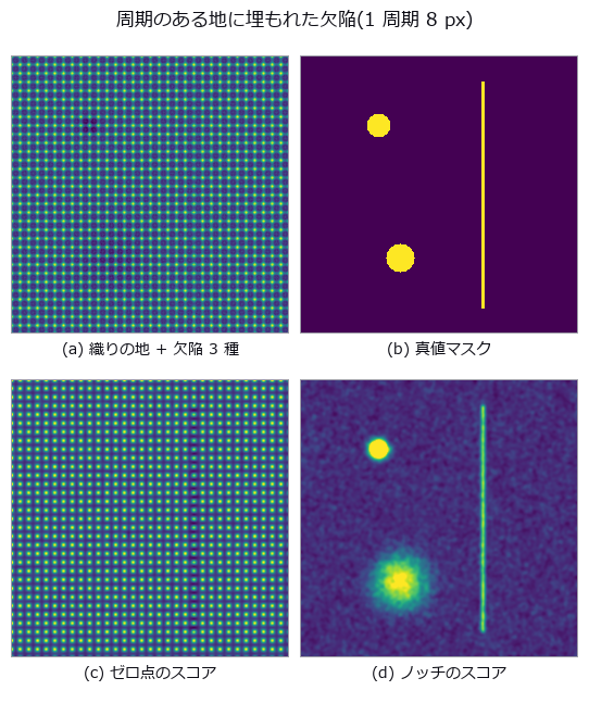
↑ Defects Buried in a Periodic Background — What a Pooled ROC Hides ―― Three defect classes (thread break, stain, dim patch) buried in a weave of period 8 px, with the detector’s score map and per-class ROC curves side by side. The everyday recipe ‘notch out the grid, remove low frequencies’ pools to an AUC of 0.8113 and looks like a pass, but the dim-patch class alone scores 0.4746, worse than chance. The one line that removes low frequencies was deleting the defect along with the lighting; drop it and the class recovers to 0.9998.

↑ The measurement (figure labels are in Japanese; the numbers are the same)
py -3.11 examples/poc_fabric_defect.py
Source: examples/poc_fabric_defect.py
7. Digging Where the Sound Says — A Clean Correlation Still Digs in the Wrong Place
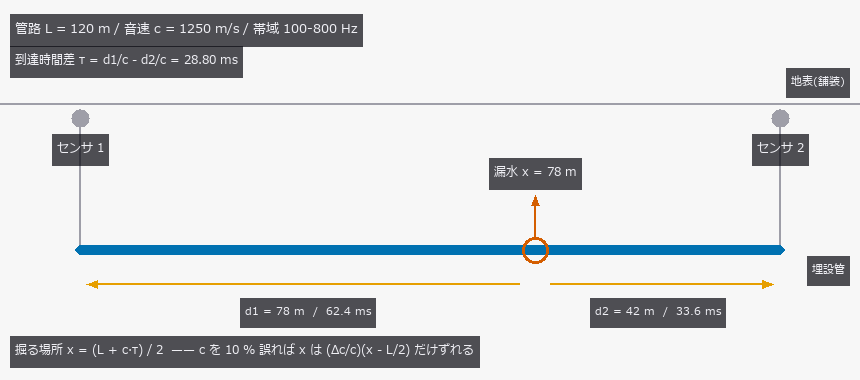
↑ Digging Where the Sound Says — A Clean Correlation Still Digs in the Wrong Place ―― Locating a leak in a 120 m buried main from the arrival-time difference at two sensors, with the source, sound speed, attenuation and reflections all planted as ground truth. With the true sound speed the estimate lands within 0.0107 m at 0 dB SNR (1.2x the Knapp-Carter bound of 0.0091 m); the threshold was predicted at -20.1 dB but measured at -12.5 dB, below which the error jumps to 36.0 m — the whole search window. Yet a 10 % error in the assumed sound speed alone moves the dig by 1.798 m (against the predicted (dc/c)(x-L/2) = 1.800 m), and on a pipe that changes from ductile iron to plastic mid-run the time difference is exactly zero, so iron, plastic or their average all miss by 18.001 m: no calibration of a single speed can fix a factor multiplying zero. The reflection prediction failed — GCC-PHAT beat the plain correlation by only 10 %, because 0.121 m of its 0.121 m RMS is bias, and whitening acts on the magnitude while the delay lives in the phase.
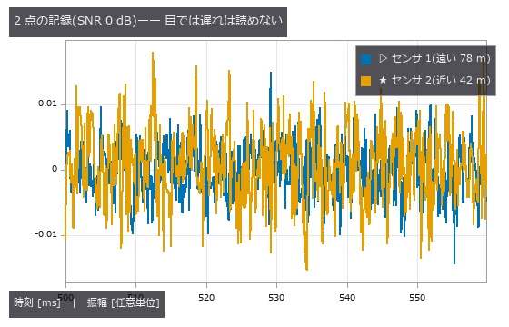
↑ The measurement ―― 同じ漏水源に既知の遅れ 28.80 ms・距離に応じた減衰・独立な広帯域雑音を乗せた。 (figure labels are in Japanese; the numbers are the same)
py -3.11 examples/poc_leak_localization.py
Source: examples/poc_leak_localization.py
Ops used (notes): arrow · bandpass · coherence · correlation_score · phase_rad · text_box · transfer_function
8. Fusing thermal, vibration and geometry for machine health — three sensors, one fact
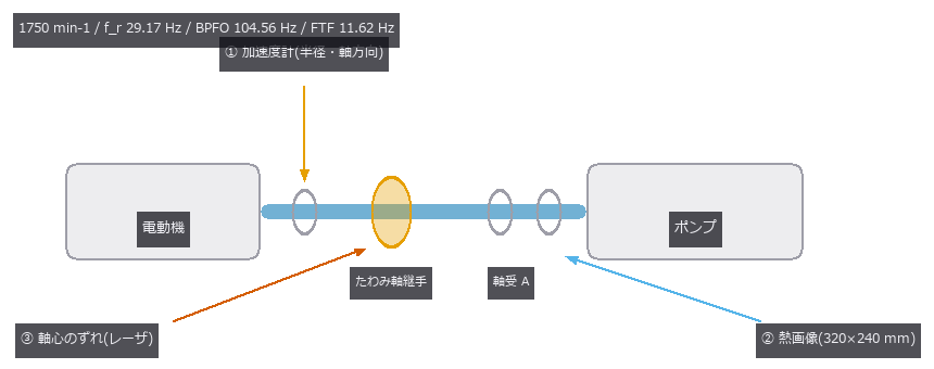
↑ Fusing thermal, vibration and geometry for machine health — three sensors, one fact ―― Six states of a rotating machine (healthy, misalignment, unbalance, outer-race spall, poor lubrication, looseness) are built from closed-form bearing defect frequencies, the exact steady fin-equation solution for the casing temperature, and a planted shaft offset, then classified from three sensors. Fused accuracy is 100.0 % — but vibration alone is also 100.0 %: thermal and geometry add nothing. Misalignment reaches 100.0 % from any single sensor (correlations with the true severity 0.843 / 0.841 / 0.978 — three faces of one number), while thermal alone can never separate healthy, unbalance and looseness (48/48 confusions inside that trio) and dropping vibration takes them from 100.0 % to 50.0 % / 31.2 %. Fusion only earns its keep once vibration breaks: at noise sigma 1.6 it lifts 45.8 % to 78.1 %. The cliffs were predicted on single features: the 0.5X order bin needs T > 2/f_r = 68.6 ms (measured d’ 2.45 -> 4.32 across the 50 -> 70 ms step), the thermal spread dies past the 66 mm half-diameter (d’ 0.00 at 96 mm pitch). The sideband prediction 1/T < FTF = 86.1 ms was wrong; the peak-reading window condition 1.2/FTF = 103 ms is the right one.
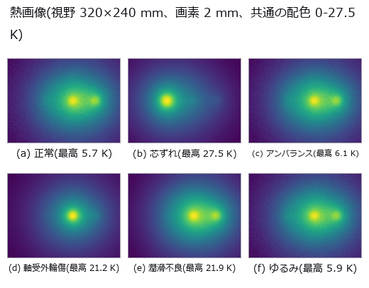
↑ The measurement ―― 軸受外輪傷は狭く熱く、潤滑不良は広く熱い。最高温度だけ見ると同じ顔になる。 (figure labels are in Japanese; the numbers are the same)
py -3.11 examples/poc_machine_condition_fusion.py
Source: examples/poc_machine_condition_fusion.py
Ops used (notes): angle_between_lines · arrow · bearing_defect_frequencies · blob_label · distance_point_line · ellipse · fuse · jitter · mat_pinv · rounded_rect · spectrum · stat_correlation · synthesize_bearing_signal · text_box
9. Reading a Binary Matrix Code — Geometry Always Dies First

↑ Reading a Binary Matrix Code — Geometry Always Dies First ―― A code with QR-style layout and random data bits (no error correction), damaged by blur, tilt and occlusion, with the raw bit error rate counted directly. The nulls sit at chance (0.526 / 0.507) while the reader scores 0.0000. Cliffs: 78 degrees of tilt, two modules of finder-pattern occlusion; run beside the condition that receives the true homography, localisation is always the stage that fails first.
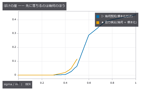
↑ The measurement ―― 自力検出の線は sigma/m 0.50 を最後に途切れる(0.60 では位置検出パターンが見つからない)。標本化はそこでまだ BER 0.07 で読めている。 (figure labels are in Japanese; the numbers are the same)
py -3.11 examples/poc_matrix_code_reading.py
Source: examples/poc_matrix_code_reading.py
Ops used (notes): adaptive_gauss_thresh · corner_response · illuminate · otsu · sk_sauvola
10. Can Display-Inspection Moire Be Told From Real Non-Uniformity?
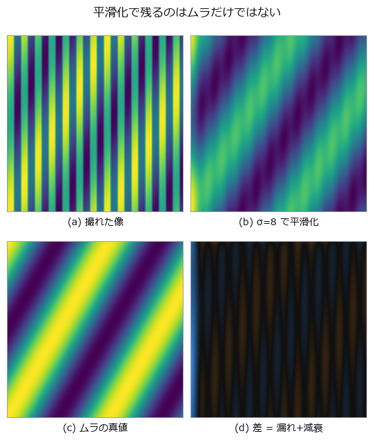
↑ Can Display-Inspection Moire Be Told From Real Non-Uniformity? ―― Moire from the interference of the display’s stripes with the camera’s pixel grid, overlaid on genuine luminance non-uniformity in one image. At a smoothing σ of 8 px the total error is +0.9 %, made of +8.3 % moire leakage cancelling -7.4 % attenuation of the real defect. At k = 0.67 the fundamental beat looks safe, yet the third harmonic lands in the defect band and the leakage reaches +202.6 % of the true value.
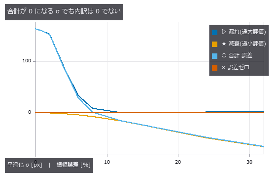
↑ The measurement ―― σ≈8 px で漏れと減衰が釣り合う。合計だけ見ると「良い測り方」に見える。 (figure labels are in Japanese; the numbers are the same)
py -3.11 examples/poc_moire_screen.py
Source: examples/poc_moire_screen.py
Ops used (notes): background_flatten · fft_image · gauss_image · reflect
11. Print Misregistration from the Sheet — A Halftone Is a Lattice, So the Answer Is Not Unique
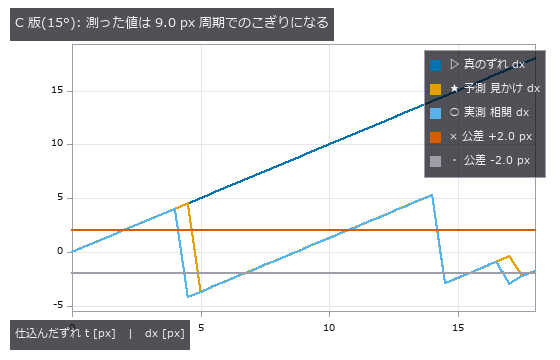
↑ Print Misregistration from the Sheet — A Halftone Is a Lattice, So the Answer Is Not Unique ―― Measuring print misregistration from the printed sheet. Four CMYK plates carry the conventional screen angles (C 15, M 75, Y 0, K 45 degrees) at 133 lpi scanned at 1200 dpi, giving a screen pitch of 9.02 px, and each plate is displaced by a known amount. The central claim is geometry: a halftone is a lattice, so correlation recovers not the displacement d but d modulo the screen lattice. Along the lattice axes that limit is p/2 = 4.51 px and along the diagonal p/sqrt(2) = 6.38 px; beyond it the measurement folds back. Stated in closed form before measuring, it matches at 144 of 148 points (four plates by 37 sweep positions) to within 0.1096 px. The four exceptions are ties on the boundary of the fundamental cell, with at most 0.165 px of margin, and reducing modulo the lattice makes every point agree: the estimator is not wrong, it returns one of the lattice-equivalent answers, and two independent estimators fold identically. The consequence is concrete. A true displacement of 9.64 px, 4.8 times the 2.0 px tolerance, appears as 1.09 to 3.32 px depending only on the screen angle, so two of the four plates look like they pass — from one sheet displaced by one amount. The null baseline, the centroid of ink, does not fold but loses its scale: the slope follows the closed form k = 1 - beta, where beta is the ink of the flat background over the total ink, predicted 0.3983 against 0.3711 measured. One effect was not predicted at all: a 0.9864 px ripple at the screen pitch, caused by rows of dots entering and leaving at the window edge, which a tapered-window control drops to 0.0048 px. Switching to an FM (stochastic) screen removes the folding entirely, with an error of at most 0.0029 px across the whole sweep, which places the blame on the periodicity of the AM screen rather than on the estimator, at the cost of 0.91 times the contrast. A window containing a registration mark reads correctly to 0.0823 px, but with 0.600 % paper stretch and 0.120 degrees of plate rotation the error grows linearly with distance at 0.006319 px per px and exceeds tolerance from 316.5 px predicted, 322.5 px measured — 44 % of the sheet. Two rulers reverse the ranking: raw correlation is the most accurate at 0.0071 px yet agrees with the pass/fail verdict only 67.6 % of the time, while low-pass filtering agrees 89.2 % of the time at 94 times the error; a two-stage estimator that picks the representative with the blunt method and refines with the sharp one wins both, and it fails exactly at the points where the coarse error exceeded the cell radius of 4.511 px. The synthesiser itself was a trap: at 150 lpi and 1200 dpi the pitch is exactly 8.00 px, every dot samples in phase, and the centroid jumps 1.4 px for each 0.5 px of displacement — avoiding the integer ratio is the fix, not supersampling. Finally, an operator used outside its domain failed confidently: fs.frame_align returned inlier_ratio 1.00 and rms_px 0.645 while missing the true (0.00, +1.30) by 80.85 px, and the answer was not even a lattice vector. That finding was fixed in the operator: its docstring now records the measurement, and the vote histogram’s runner-up over winner is returned as vote_margin — 1.000 on this halftone against 0.143 on a star field, where the agreement ratio is 1.00 in both.
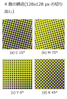
↑ The measurement ―― スクリーン角が違うので格子の向きが違う。ピッチはどれも 9.02 px。同じ物理的なずれでも、この格子の違いが「見かけのずれ」を版ごとに変える(5 節) (figure labels are in Japanese; the numbers are the same)
py -3.11 examples/poc_print_registration.py
Source: examples/poc_print_registration.py
Ops used (notes): fly_hex_lattice · frame_align · inlier_ratio · peak_subbin · piv_cross_correlate
12. How Faint a Defect Can Still Be Found — Planting a Known Truth in a Real Background

↑ How Faint a Defect Can Still Be Found — Planting a Known Truth in a Real Background ―― The usual way to estimate “how faint a defect can we still catch” is to measure the limit on a synthetic image: a flat field plus white noise. This exhibit measures how optimistic that estimate is, while keeping an exact ground truth. The backgrounds are three CC0 photographs (brick / grass / gravel); what is planted into them is a Gaussian defect of known position, width and amplitude. The control is a synthetic field whose residual sigma — the variation the detector actually sees — is matched to the real one, so the amount of noise is equal and only structure differs. The verdict is the smallest amplitude at which the planted position becomes the peak of the response; no threshold is involved, so per-image normalisation inside an operator cannot skew it. Matching the noise is not enough: the real backgrounds raise the floor by 2.03x to 3.47x. What sets the floor is structure, not noise. The gap survives all 18 knob settings (three background windows x two defect sizes x three grounds, 1.72x-4.56x) and both detectors — a matched filter and fullseye’s laplace_of_gauss. A prediction that failed: “the gap widens for larger defects” turned out to be an artefact of the amplitude grid — on 34 steps the two sizes round to different grid points, on 60 steps both land at 3.30x. The grid is a knob too. “Real data is position-dependent” is also wrong: the spread of the floor across positions is 16.8x on brick but 2.4x on grass and 3.3x on gravel, indistinguishable from the 3.3x of the matched synthetic control. What creates the spread is the mortar lattice — a structure — not the fact that the image is a photograph. And the null model wins on a single metric. Taking the brightest raw pixel, with no background removed, localises the defect at 0.65x-0.90x the amplitude the matched filter needs, because the matched filter amplifies the background’s structure too; false alarms on a defect-free surface tie at 0 on brick. The two separate the moment the lamp drifts by 2 %: the null model fires 10.3 times per 10,000 pixels while the matched filter stays at 0.0, because a raw-pixel threshold is an absolute brightness. Count localisation, false alarms and drift separately, or a useless detector can be made to win.
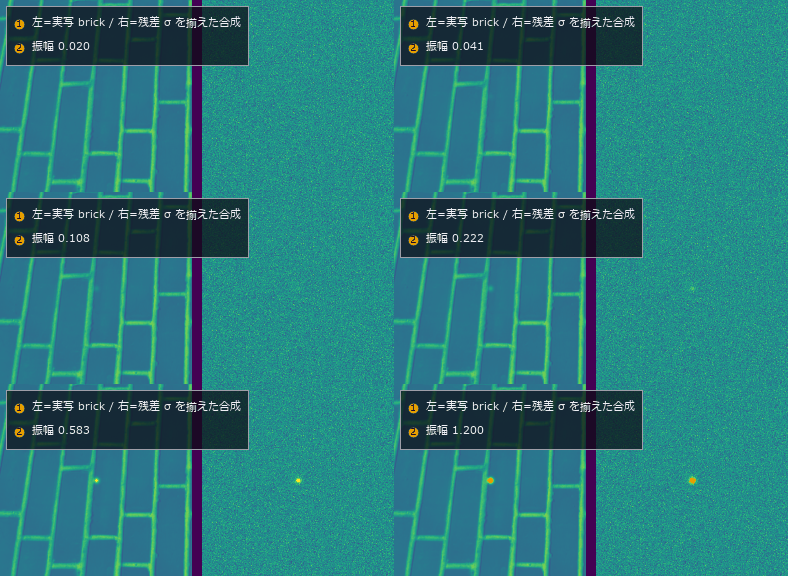
↑ The measurement ―― 同じ欠陥を振幅 0.02 から 1.20 まで上げていく。左=実写の brick、右=残差 σ を揃えた合成の地。雑音の量は同じなのに、右のほうが先に見えてくる。 (figure labels are in Japanese; the numbers are the same)
py -3.11 examples/poc_real_defect_floor.py
Source: examples/poc_real_defect_floor.py
Ops used (notes): annotate_inset · annotate_legend · laplace_of_gauss · reflect
13. Rotating Real Textures — Rotation Invariance Holds Only Where It Is Not Needed
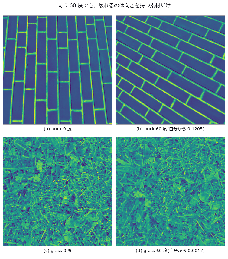
↑ Rotating Real Textures — Rotation Invariance Holds Only Where It Is Not Needed ―― Three real textures (brick, grass, gravel, all CC0) rotated by known angles, measuring how far the descriptor drifts from itself. The benchmark is set before measuring: the smallest distance between materials, 0.01250 between grass and gravel, is the resolution of the task, and any rotation drift beyond it means a rotated sample is further from itself than from a different material. The anisotropic brick drifts 0.0433 at five degrees and 0.1205 at sixty, 9.6 times the resolution, while grass and gravel stay at 0.0005 to 0.0024, effectively invariant. Two controls isolate the cause: interpolation alone, measured by rotating plus seven and back minus seven degrees, contributes 0.03685 for brick, and an exact ninety-degree rotation with no interpolation at all still gives 0.08501, or 6.8 times the resolution. Anisotropy can be measured independently and explains the ranking: the global concentration of gradient orientation is 0.309 for brick against 0.027 and 0.029 for the others. Switching to rotation-invariant encodings brings brick from 9.64 down through 5.49 to 1.72 — never below one — while the isotropic pair improves tenfold, from 0.17 to 0.02. LBP’s rotation invariance applies to the cyclic shift of a local pattern; it cannot remove the orientation distribution of the material itself.
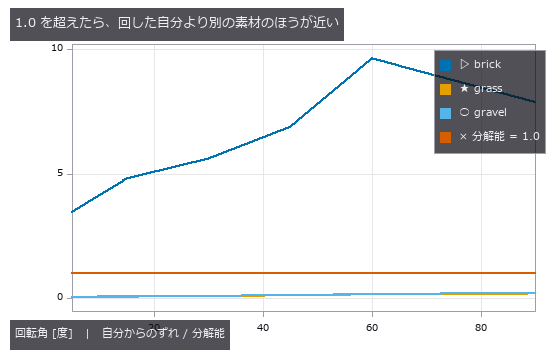
↑ The measurement ―― brick だけが 1 を大きく超える(最大 9.6 倍)。 (figure labels are in Japanese; the numbers are the same)
py -3.11 examples/poc_real_texture_invariance.py
Source: examples/poc_real_texture_invariance.py
Ops used (notes): cooc_feature_matrix · reflect · sk_lbp
14. Sorting mixed waste by material — what a preprocessor can erase is decided by algebra

↑ Sorting mixed waste by material — what a preprocessor can erase is decided by algebra ―― Fragments on a belt carry material, dirt, wetness, tilt and occlusion in known amounts, imaged in 64 SWIR bands. Per-fragment degradation is closed form, s(l)=gR(l)exp(-wA_w(l))+(au(l)+c), so invariance can be predicted before measuring: the spectral angle is invariant to the multiplicative g (0.995 to 0.990 as dirt goes 0 to 0.8; 0.993 at 70 degrees of tilt), and a second derivative annihilates the linear baseline (raw SAM falls 0.995 to 0.827 under an additive baseline while the derivative stays at 0.995 at every level). Two predictions failed: wetness is largely removed by the second derivative (0.818 against 0.282 for raw SAM) because a second derivative weights Gaussian bands by 1/sigma^2 ((43/70)^2 = 0.37), and continuum removal beats raw SAM while the baseline is weak (0.983 vs 0.865) but loses once it is strong (0.736 vs 0.827). Featureless metal vanishes under differentiation (recall 0.06) and a flatness gate restores it to 0.98.

↑ The measurement ―― PP と PE は骨格が同じ(-CH2-)なのでわざと似せてある。 (figure labels are in Japanese; the numbers are the same)
py -3.11 examples/poc_recycling_sorting.py
Source: examples/poc_recycling_sorting.py
Ops used (notes): overlay_labels · spectrum
15. Power loss from solar-cell EL images — dark is not the same as inactive

↑ Power loss from solar-cell EL images — dark is not the same as inactive ―― A crystalline-silicon cell (100 fingers, 3 busbars, 70 grains) is rendered in closed form as an EL image with two electrically isolated regions (true inactive area 4.77 %), 5 cracks and 8 finger interruptions, then imaged through cos^4 vignetting and photon noise. The zero-point global threshold reports a dark-pixel fraction of 21.7 % as the inactive area, but 42 % of those pixels are fingers and busbars and 33 % are grains and vignetting; only 20 % are truly inactive. Dividing out the grid with row/column profiles and gating each defect type separately gives 4.61 % (-0.15 points), crack recall 0.88–1.00 and 8/8 interruptions. Because sk_frangi normalises by the per-image maximum, a calibration line only fixes the scale if it is the strongest ridge in the image (a line like the real cracks responds 0.69, a 3 px black line 1.00); without calibration the defect-free cell produces 147 px of false cracks. From grain contrast c=0.24 false cracks and swallowed interruption bands start together, and the crack-width cliff at 1.25 px follows the linear width-times-depth rule (predicted 1.38 px).

↑ The measurement (figure labels are in Japanese; the numbers are the same)
py -3.11 examples/poc_solar_el_inspection.py
Source: examples/poc_solar_el_inspection.py
Ops used (notes): aug_vignette · blob_features · blob_label · blob_select · gaussian · gray_closing · hysteresis_threshold · lines_gauss · otsu · sk_frangi · sk_skeleton · total_length · vignette
16. Solder fillet AOI — three ring lights are a 3-level tilt quantiser, and 70 % of the fillet height sits in the dark
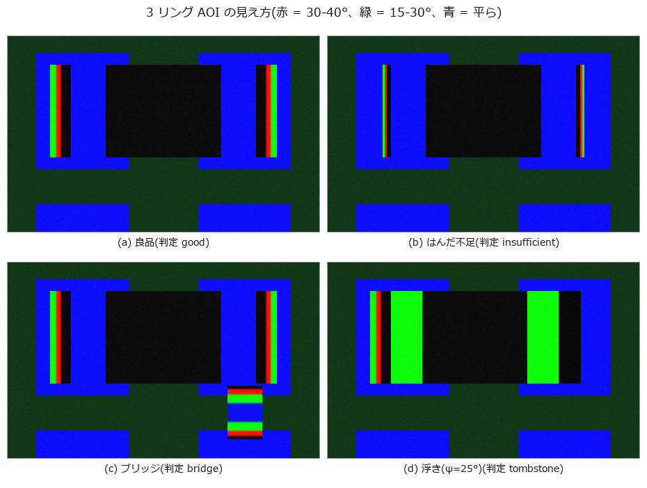
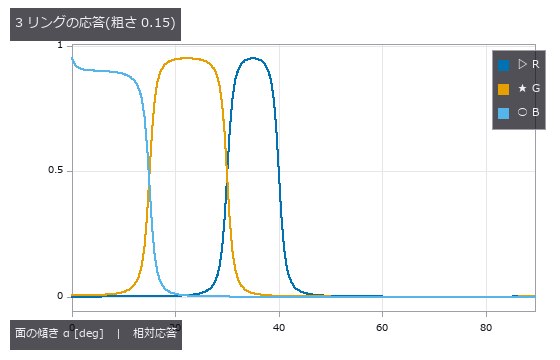
↑ Solder fillet AOI — three ring lights are a 3-level tilt quantiser, and 70 % of the fillet height sits in the dark ―― A 1608 chip’s pads and terminations carry circular-arc fillets fixed by contact angle and cross-section area; three ring lights at different elevations (red 30-40°, green 15-30°, blue 0-15° of surface tilt) are integrated over a GGX lobe to synthesise the AOI image, and joints are graded good / insufficient / bridge / tombstone. With an 18° contact angle the concave arc rises to 72° at the wall, so even the lowest ring sees only 28.8 % of the height (predicted): naively integrating the band tilts recovers 0.284 of the true height. Extrapolating the arc to the wall from the positions where the colour changes lands at +1.7 % ± 5.3 % for free arcs, but once extra solder pins the toe at the pad edge it drifts to -42.3 %. A 0.16 mm placement offset steepens the toe past 30°, the green band vanishes and a good joint is called insufficient although its true height has risen (predicted 0.16 mm; the truth only fails at 0.28 mm). Surface roughness, against expectation, does not move the dark edge; it breaks at roughness 0.5 together with the loss of the red band and at 0.6 the whole fillet drops below the dark threshold. The zero point (Lab distance of the pad mean colour) is 100 % right under reference conditions yet flags 56 % of good joints and 68 % of bridges once offset, roughness and lighting vary — no discrimination — while the arc-based grading scores good 98 % / insufficient 98 % / bridge 100 % / tombstone 88 %, the misses all being lifts of 8.7-11.0°.
↑ The measurement ―― 鏡面なら窓の端が階段になる。傾き 40° を超えるとどのリングも届かない。 (figure labels are in Japanese; the numbers are the same)
py -3.11 examples/poc_solder_fillet_aoi.py
Source: examples/poc_solder_fillet_aoi.py
Ops used (notes): access_channel · blob_features · blob_label · blob_select_largest · brdf_microfacet · illumination_design · intensity · rgb_to_lab · trans_from_rgb
17. Is the Process in Control, and Is It Capable? — Statistical Process Control from Closed-Form Alone
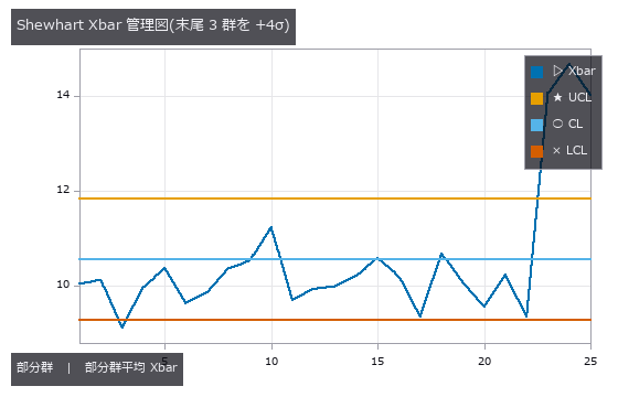
↑ Is the Process in Control, and Is It Capable? — Statistical Process Control from Closed-Form Alone ―― A series of dimensions and defect counts measured by machine vision, fed through four SPC ops that use no learning at all (each a textbook closed-form with an exact identity to check against). The Xbar-R chart catches a +4σ shift planted at the tail across 4 subgroups at once (n=5 constants A2/D3/D4 = 0.577/0.000/2.115, ISO 8258); CUSUM catches a +0.8σ sustained drift that Shewhart 3σ never flags, at #45 (right after the drift starts). Process capability separates “capable” from “capable at the current centre”: centred on the spec midpoint Cpk = Cp = 1.307, shifted by +1 Cpk = 0.981 < Cp. Multivariate T² folds the simultaneous drift of three correlated measurements into one verdict (UCL from the F-distribution). As with image restoration, a process running and a process in control are measured separately.
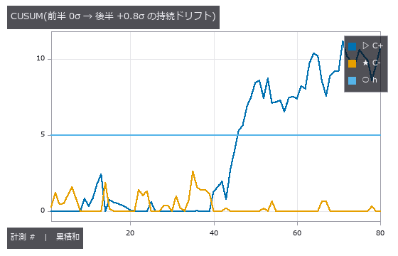
↑ The measurement ―― Shewhart 3σ は 0 件、CUSUM は #46(ドリフト開始の直後)で h=5 を超えて警報。 (figure labels are in Japanese; the numbers are the same)
py -3.11 examples/poc_spc.py
Source: examples/poc_spc.py
Ops used (notes): spc_capability · spc_cusum · spc_hotelling_t2 · spc_xbar_r
18. How Much Camera Thermal Drift Costs a Dimensional Measurement

↑ How Much Camera Thermal Drift Costs a Dimensional Measurement ―― A 40 mm square measured by a camera whose focal length, mount and principal point drift with temperature ΔT, the error split into a + b·R in image radius. At ΔT = 15 K the constant term is +224.5 ppm (the single-cause control gives +225.3 ppm). Drift rises above the noise floor (23 ppm for a 25-frame average) only from ΔT = 1.6 K; below that, the honest report is that no temperature effect is visible.
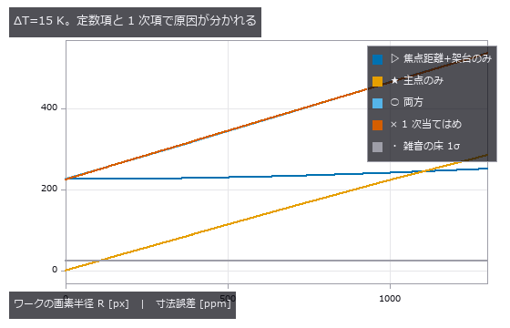
↑ The measurement ―― 焦点距離ドリフトは R に依らない。主点ドリフトは R に比例(歪みを外す中心がずれるため)。 (figure labels are in Japanese; the numbers are the same)
py -3.11 examples/poc_thermal_drift_metrology.py
Source: examples/poc_thermal_drift_metrology.py
19. A Thermal Image Is Not a Temperature Image — Emissivity, Reflection, and an Uncertainty That Does Not Add
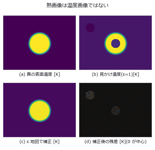
↑ A Thermal Image Is Not a Temperature Image — Emissivity, Reflection, and an Uncertainty That Does Not Add ―― Take a thermal camera’s digital numbers all the way back to temperature, with the truth planted: L = tau [ eps L_bb(T_obj) + (1-eps) L_bb(T_refl) ] + (1-tau) L_bb(T_atm). The floor is measured first — 1.75e-06 K round trip, 6.28e-03 K with quantisation, 2.71e-02 K with NETD — and re-measured off the calibration knots, because at exactly 350.0 K the error came out identically zero and calling that a floor would be a lie. The closed form was printed before measuring, and it was wrong: the naive Planck exponent n = c2/(lambda T) misses the numerical derivative by up to 16.6 %, and the culprit is not the choice of effective wavelength but the missing e^x/(e^x - 1) factor; with it the error is 0.00 %. The direction of the cliff was wrong too. ‘Colder is steeper’ was printed, but the absolute error grows with temperature (0.233 K at 305 K against 16.907 K at 800 K for a 5 % emissivity error), with a measured log-log slope of 2.717 that decomposes exactly as T/n = 1.741 plus a reflection term of 0.977 — the closed form had said so all along and was misread. ‘Colder is steeper’ does hold when the error is scaled by the rise above ambient, but the culprit is different: the emissivity term only moves 1.40 times and converges, while getting the reflected temperature wrong moves 972 times. The centre of the exhibit is that uncertainty does not add. With emissivity 0.60 +/- 0.05, reflected temperature 300 +/- 5 K and a correlation of +0.7, a ‘95 % interval’ actually contains the truth 88.03 % of the time under independent root-sum-square and 94.44 % under a correlated Monte Carlo — and the floor was measured first, since at zero correlation the two agree (95.03 % and 94.52 %), so the gap is the neglected correlation itself and nothing else. The RSS interval is 20.2 % too narrow; at a correlation of -0.7 it becomes 99.64 %, too wide. Assuming independence is neither the safe side nor the dangerous side — it is the unknown side. On an acceptance decision over 40000 trials the false-accept rate runs 8.03 % ignoring uncertainty, 0.81 % with RSS and 0.14 % with the correlated Monte Carlo: RSS lets through 5.6 times as many bad parts. Of eight unit and convention mistakes, three raise and five pass silently — and the same mistake (writing the reflected temperature in Celsius) passes quietly at emissivity 0.95 while raising at 0.10, so whether the code stops depends on the scene, not on the kind of error. In the image itself a bolt at emissivity 0.10 sitting directly over the heat source reads 62.3 K colder than the painted metal around it at the same 375.0 K: the hottest place looks the healthiest. Correcting with an emissivity map recovers 375.0 K, but trades bias for variance — the residual is 6.4 times noisier on the bolt than on the paint. Along the way a real defect was found and fixed: the robust noise estimate collapses to zero on integer digital numbers, and the downstream point-target detector was silently returning nothing at all.
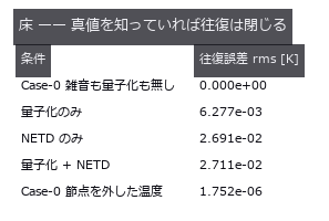
↑ The measurement ―― LWIR・350 K・ε=0.95。校正表と直接積分の相対差は最大 8.9e-16。以下の誤差はすべてこの床の上。 (figure labels are in Japanese; the numbers are the same)
py -3.11 examples/poc_thermal_radiometry.py
Source: examples/poc_thermal_radiometry.py
Ops used (notes): beer_lambert_transmittance · interp_linear · mat_eigh · noise_sigma · photon_uncertainty · poly_fit · stat_correlation · stat_covariance · stat_describe · stat_histogram
20. Depth of a Subsurface Defect by Pulsed Thermography
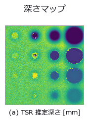
↑ Depth of a Subsurface Defect by Pulsed Thermography ―― Surface temperature after a flash, generated from the exact 1-D heat-conduction solution, with delamination depth estimated from the image sequence. Where the diameter is at least four times the depth the estimate lands within a few percent; at 0.5 mm deep and 2 mm across it is off by +627 %. The cause is not lateral diffusion but the fitting window: shortening it from 25 s to 4 s brings that case back to -9 %.
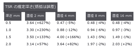
↑ The measurement ―― 右下三角(直径が深さの 4 倍以上)は数 %。左上は横拡散で壊れる。 (figure labels are in Japanese; the numbers are the same)
py -3.11 examples/poc_thermography_ndt.py
Source: examples/poc_thermography_ndt.py
21. Veiling Glare Breaks Contrast Measurement — MTF Passes While Black Level Fails
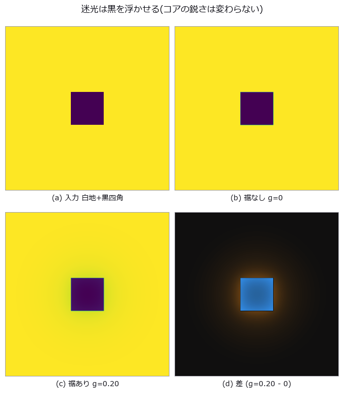
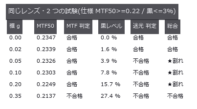
↑ Veiling Glare Breaks Contrast Measurement — MTF Passes While Black Level Fails ―― A PSF whose core stays sharp while only its tail is made heavier, with the slanted-edge MTF and the black level of a dark square measured on the same image. Raising the tail fraction from 0 to 0.20 moves MTF50 from 0.2347 to 0.2249 cyc/px (-4.2 %, still passing) while the black level goes from 0.0 to 15.7 % (failing). A ±16 px measurement window captures only 6 % of the tail’s energy; a glare figure means nothing until the measurement extent is declared.
↑ The measurement (figure labels are in Japanese; the numbers are the same)
py -3.11 examples/poc_veiling_glare.py
Source: examples/poc_veiling_glare.py
Ops used (notes): airy_pattern · create_funct_1d_pairs · derivate_funct_1d · get_y_value_funct_1d · invert_funct_1d · mtf_diffraction · psf_to_mtf
22. Naming the Damaged Roller from a Period — You Run Out of Evidence Before You Reach the Cliff
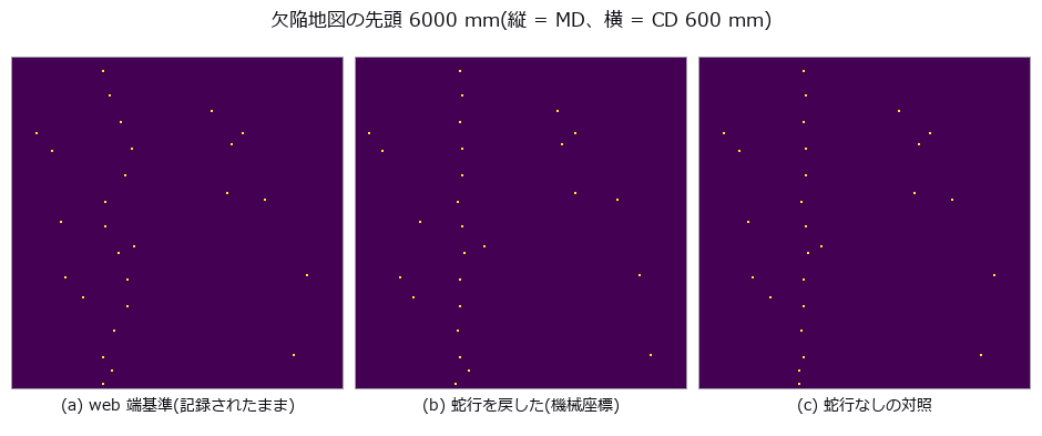
↑ Naming the Damaged Roller from a Period — You Run Out of Evidence Before You Reach the Cliff ―― In roll-to-roll production of film, battery electrode, copper foil and paper, a single scar on a conveying roller prints itself onto the web once per roller circumference. Can the machine-direction spectrum of a defect map recover that circumference and name the culprit against a table of piD? Reading the naive spectral maximum names a real but innocent roller: an impulse train has a comb whose harmonics are as tall as the fundamental, so the maximum grabs C/2 = 235.62 mm, and that lands on the cooling roller at 314.16 mm in the table. A circumference that exists nowhere would be caught; one that exists elsewhere in the table passes review. That error stays at 235.9 mm as the miss rate goes from 0 to 50 % — a constant error is not evidence of robustness, it is the same mistake repeated. The fix is fail-closed: take the lowest frequency at which harmonics k=1..3 all stand. The null baseline, the median spacing between detected defects, is right when detection is perfect (-0.03 mm) but at a 40 % miss rate it errs by 472.1 mm and the mean by 813.5 mm, while the comb method holds at 3.2 mm — a missed defect removes amplitude without moving phase. A 25 mm meander, uncorrected, splits one roller’s defect line into two across the web (periodic defects remaining in the lane fall from 100 % to 44 %), yet the MD spectrum is bit-for-bit unchanged: meander only breaks methods that cut lanes in the cross direction. Sixty control trials with only healthy rollers give a 1.7 % false-positive rate, and the floor is not zero — the healthy side reaches 3.99 times the band median, above the 2.5 threshold on its own, so what actually holds the line is the demand that every harmonic stand. There are two cliffs. The prediction L_crit = C^2/dC = 14137 mm matches the measured resolution cliff at 14000 mm, a ratio of 0.99. But the detection cliff, the shortest record that still always reports, is 17000 mm — longer. Shortening the record makes you say nothing before it makes you say the wrong roller, so the cliff Rayleigh predicted correctly is never reached. The criterion itself needed repair: at 24 trials a clean 0 % existed, at 120 trials 2 % survives even at the longest record, so 0 % was a small-sample artefact rather than a floor. The most frequent wrong answer, at seven of nine sweep points, is the cooling roller, and 471.24 / 314.16 = 1.500 is exactly 3:2: an integer ratio inside the table gives the comb method a misidentification of its own. The two gaps this PoC found have since been filled: fs.point_spectrum takes a periodogram straight from event positions and carries its own resolution in the return value, and fs.peak_subbin refines a peak below the bin without clamping the shift, since a vertex further than half a sample away means the index was not a maximum at all.*

↑ The measurement ―― 見逃しは位相を飛ばさないので、櫛の山は低くなるだけで動かない。 (figure labels are in Japanese; the numbers are the same)
py -3.11 examples/poc_web_roll_periodicity.py
Source: examples/poc_web_roll_periodicity.py
Ops used (notes): cepstrum · find_peaks · local_min_max_funct_1d · median · peak_subbin · point_spectrum · smooth_funct_1d_gauss · spectrum
23. Weld Bead From a Laser-Triangulation Profile — The Sin of Writing 0 Where Nothing Was Measured
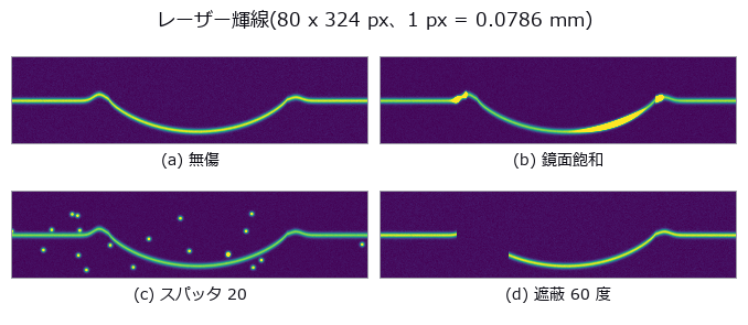
↑ Weld Bead From a Laser-Triangulation Profile — The Sin of Writing 0 Where Nothing Was Measured ―― The profile h(x) recovered from the row position of a single laser line, with reinforcement height, width and undercut read off it. The centroid beats the null (integer argmax per column) by 9.3x, and with zero noise the log-parabola is exact to machine precision, 12 orders better than a plain parabola; at 1 % noise the two are 0.00272 versus 0.00260 mm, indistinguishable. Five spatter points break all three estimators together to 0.11 mm (40x); what matters is not refinement but which peak you pick.
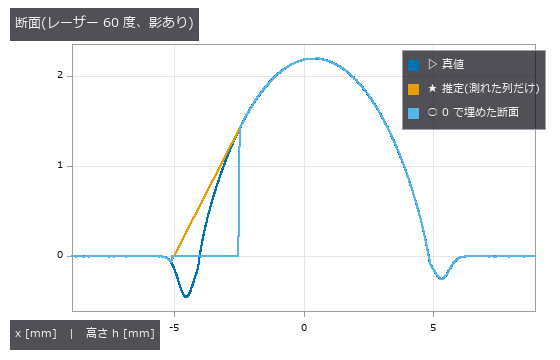
↑ The measurement ―― 0 で埋めた線は影の区間で h=0 に張り付き、左のアンダーカットが消えて偽のつま先ができる。 (figure labels are in Japanese; the numbers are the same)
py -3.11 examples/poc_weld_bead_profile.py
Source: examples/poc_weld_bead_profile.py
Ops used (notes): gen_measure_rectangle2 · measure_pos · median · smooth_funct_1d_mean
24. Light-section scanning of a weld bead — resolution and occlusion share one knob
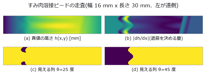
↑ Light-section scanning of a weld bead — resolution and occlusion share one knob ―― A fillet-weld cross-section is built in closed form with convexity, leg lengths, throat and undercut depth varied along the weld line by known functions, then the triangulation angle is swept from 15 to 70 degrees. Height resolution improves as 1/sin(theta) while any face rising steeper than cot(theta) hides in its own shadow, so the far parent plate turns away exactly at the predicted 37.0 degrees and the far undercut starts vanishing earlier, at 20.8-34.5 degrees (the deeper the groove, the sooner). The dangerous parts are that at 28 degrees every cross-section still reports a value while 25 % of the groove span is unmeasured and the depth reads 27 % shallow, and that raising the angle further drops the deepest cross-sections out of the average (true mean drifting 0.260 to 0.047 mm) — a survivorship bias; the optimal angle differs per measurand at 20 / 24 / 36 / 64 degrees.
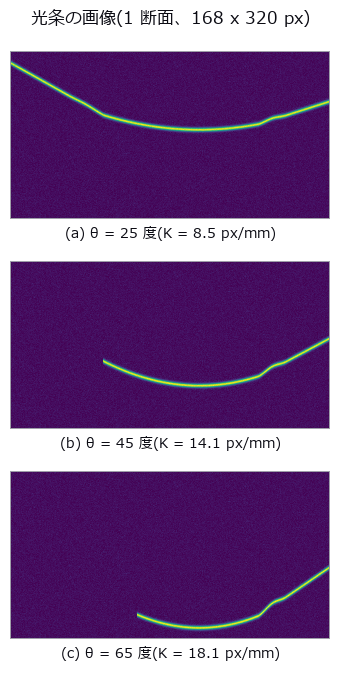
↑ The measurement ―― θ を大きくすると高さの伸び K が増えて分解能は上がる(輝線の起伏が大きくなる)が、左半分の輝線が消えていく。 (figure labels are in Japanese; the numbers are the same)
py -3.11 examples/poc_weld_bead_scan_angle.py
Source: examples/poc_weld_bead_scan_angle.py
Ops used (notes): esdf · fit_plane_3d · intersect_planes · lines_gauss · normals_from_depth · occupancy_grid · query_distance
25. Porosity in Weld Radiographs — Closing With the Share of Images Misgraded by One Class

↑ Porosity in Weld Radiographs — Closing With the Share of Images Misgraded by One Class ―― A radiograph drawn in closed form with Beer–Lambert: 10 mm plate, arc-shaped reinforcement, spherical pores, plus scatter, unsharpness and film grain. The fixed-threshold baseline counts the weld toe as pores (124 blobs, total area 15.19 mm² against 7.93 true). The detection cliff is predictable from CNR = 16.12·d²: Rose’s CNR = 4 misses (0.50 mm), while the prediction that includes smoothing and the 3 px minimum area gives 0.58 mm against 0.57 mm measured. The 9 px window cap of the background-estimation op (rectangular opening) becomes a cliff: detection drops below 50 % from 2.0 mm and reaches 0 % at 2.5 mm — choosing the op chooses the measuring range. Scatter at SPR = 1 shrinks the volumetric diameter by (1+SPR)^(-1/3): -22.6 % measured against -20.6 % predicted. Images misgraded by one class: 90 % for the baseline, 23 % with the volumetric diameter.

↑ The measurement (figure labels are in Japanese; the numbers are the same)
py -3.11 examples/poc_weld_radiograph_porosity.py
Source: examples/poc_weld_radiograph_porosity.py
Ops used (notes): blob_features · blob_label · blob_overlay · blob_select · estimate_noise · gauss_image · gen_measure_rectangle2 · gray_opening_rect · identity · log_image · measure_pairs · measure_pos · median_rect · sk_rolling_ball · xsitk_grayscale_grindpeak
The Dimensional and Shape Metrology Wing — Keep Bias and Scatter Apart
To state that a part is 50.50 pixels wide, you need bias (the part that always shifts the same way) and scatter (the part that changes from shot to shot) as two separate numbers. Pass/fail is decided by bias; repeatability by scatter. Merge them into one ‘error’ and you no longer know which countermeasure to take.
The ten exhibits here hold their ground truth in closed form or analytic rendering — a signed-distance-function part, an involute gear, a roughness surface synthesised from a prescribed PSD, a white-light interferometry stack, analytic speckle, Frocht’s stress field, a perfectly symmetric synthetic skull — and then score caliper, correlation and phase readings against it.
The recurring finding is that a number without its definition cannot be compared: crack widths that differ by 0.20 mm between two distance-transform conventions, a D50 that differs by 1.66x between number- and area-weighting, an Sz that never plateaus as the evaluation area grows, an orientation index that moves 5 % depending on whether the truth is counted by fibre or by length. These are not instrument errors; they are questions of what you are comparing against.
26. Matching Full 2-D Inspection to Sampled 3-D Inspection — A Grid Overlaps Itself

↑ Matching Full 2-D Inspection to Sampled 3-D Inspection — A Grid Overlaps Itself ―― The real line has two stages: AOI images every unit from above, X-ray CT samples a few and images the inside. What the floor wants to know is how far the CT numbers follow from the AOI numbers — which is not a question about one instrument’s accuracy but about whether two instruments’ indices point at the same joint. A regular array does not match one-to-one on point positions alone: all 30 pads of a 6x5 grid have degenerate distance signatures (9 distinct ones), because the grid maps onto itself and the orientation cannot be read. Fiducials with three distinct side lengths (3600/5200/6325 um) pin rotation and reflection uniquely, and the correspondence is recovered exactly under translation, rotation and re-indexing. With that closed, AOI’s apparent void fraction correlates 0.973 with CT volume fraction and the worst five agree 5/5 — yet of the 27 parts carrying an interface-touching void (the kind that shortens life), those five catch only 19 %. Agreeing on the ranking does not mean catching the dangerous ones. The failed first attempt (Kabsch alone) is kept.

↑ The measurement ―― 直線は「面積率に比例する」という素朴な仮定。点はそこから両側へ離れる。 (figure labels are in Japanese; the numbers are the same)
py -3.11 examples/poc_aoi_ct_traceability.py
Source: examples/poc_aoi_ct_traceability.py
Ops used (notes): vol_label
27. As-built wall deviation — the bounding box measures the room’s heading, not its size
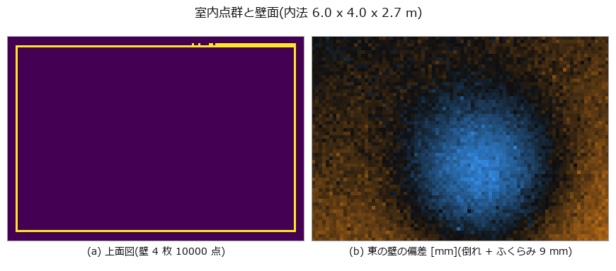
↑ As-built wall deviation — the bounding box measures the room’s heading, not its size ―― A 6.0 x 4.0 x 2.7 m indoor point cloud carries known defects: wall plumb errors of 1.20-9.00 mrad, a 5.00 mrad plan-view squareness error, and a 9 mm out-of-plane bulge. The naive axis-aligned bounding box over-reports the width by 19.1 mm, and rotating the room by just 1 deg relative to the scanner axes adds 80.1 mm (611.1 mm at 10 deg) — it is measuring W cos psi + D sin psi, the room’s heading, while the plane-pair distance stays at +2.24 mm regardless. The AABB also grows with sample size (+14.9 to +19.7 mm for 256x more points, the 2-sigma-sqrt(2 ln N) extreme-value law), so adding measurements makes it worse. Furniture outliers break the two estimators differently: least squares is off by 11x the truth at 10 % contamination (66.3 mrad vs a closed-form 63.8), while RANSAC holds to 45 % and then jumps onto the cabinet at 55 % — where the plumb error stays a harmless 0.13 mrad but the plane itself is 449.9 mm out, so one number hides the failure. A single bulge corrupts plumb (-1.258 mrad), squareness (+0.500 mrad) and the internal dimension (+2.2 mm) at once, all predicted in closed form to within 0.06 mrad.

↑ The measurement ―― 許容 ±10 mm。AABB は ψ=0.5 度で既に外れる。 (figure labels are in Japanese; the numbers are the same)
py -3.11 examples/poc_asbuilt_wall_deviation.py
Source: examples/poc_asbuilt_wall_deviation.py
Ops used (notes): aabb · angle_between_planes · angle_line_plane · distance_point_plane · fit_plane3 · ransac_plane
28. Measuring electrode breathing in microns — sub-pixel is not enough
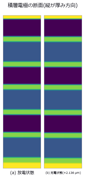
↑ Measuring electrode breathing in microns — sub-pixel is not enough ―― Electrode swelling is read from two cross-sections by tracking layer boundaries to sub-pixel accuracy. Ground truth: anode 1.00 %, cathode 0.20 %, separator 0 %, stack 480.0 -> 482.136 um (+2.136 um = +0.4450 %). Counting binarised pixels resolves 0 of 12 layers, while a fixed-threshold crossing is also sub-pixel and lands on the answer with no noise (+0.004495) — what kills it is the control group: with zero strain, an illumination offset of +0.10 alone yields -1.07e-02, a false strain 2.4x the true one and of the opposite sign, and a gain of x1.30 halves the crossings so the measurement fails outright. The gradient-peak estimator (measure_pos) stays at exactly 0.0 under both. Doubting our own ‘1.8e-14 px error’ and shifting the stack by fractions of a pixel showed that figure to be an artefact of putting the truth on pixel centres: the real error is peak locking, RMS 0.0088 / max 0.0122 px, worth 3.0 % on the anode’s strain. The cliff has two steps, and the one where boundary counts collapse arrives 5.5x earlier than the predicted 3-sigma limit.
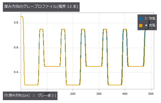
↑ The measurement ―― 境界は erf の重ね合わせで解析的に置いてあるので、真値は浮動小数点の精度で既知。 (figure labels are in Japanese; the numbers are the same)
py -3.11 examples/poc_battery_electrode_breathing.py
Source: examples/poc_battery_electrode_breathing.py
Ops used (notes): auto_threshold · gen_measure_rectangle2 · measure_pos · piv_peak_locking
29. Measuring Bilateral Asymmetry — The Symmetry Plane Gets Dragged by the Deformation
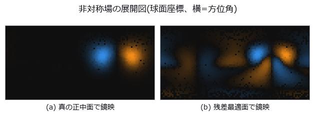
↑ Measuring Bilateral Asymmetry — The Symmetry Plane Gets Dragged by the Deformation ―― A perfectly symmetric synthetic skull with a known bulge added on one side, mirrored and overlaid. Even a perfectly symmetric specimen never scores 0: the floor drops from 1.33 mm (point-to-point) to 0.030 mm (point-to-plane) to 0.012 mm (neighbourhood smoothing). The residual-minimising plane is dragged 2.92 mm / 1.72 degrees by a 6.33 mm bulge, and 46 % of the asymmetry disappears.

↑ The measurement ―― 完全対称な標本を測った残差。点対点は点間隔がそのまま床になる。 (figure labels are in Japanese; the numbers are the same)
py -3.11 examples/poc_bilateral_asymmetry.py
Source: examples/poc_bilateral_asymmetry.py
Ops used (notes): chamfer_distance · detect_reflection_symmetry · detect_rotational_symmetry · estimate_normals · hausdorff_distance · reflect_points · reflection_symmetry_score · sample_surface · vertex_normals
30. Strain From Speckle Images (DIC)
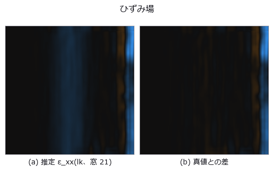
↑ Strain From Speckle Images (DIC) ―― Displacement and strain read from a speckle pair in which 3000 Gaussian spots were moved by the deformation map and redrawn, not interpolated. For a true shift of 0.37 px the window-correlation estimator (piv) is biased by 0.0002 px with 0.0022 px scatter, 167x better than the null that answers ‘no motion’. A rigid rotation manufactures several hundred µε of false strain under the small-strain definition; Green-Lagrange gives exactly 0.
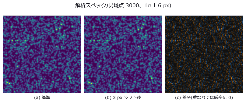
↑ The measurement ―― 変形は補間ではなく斑点の再描画。だから真値が厳密。 (figure labels are in Japanese; the numbers are the same)
py -3.11 examples/poc_dic_strain.py
Source: examples/poc_dic_strain.py
Ops used (notes): piv_cross_correlate · strain_from_displacement
31. Die tilt and TSV overlay from one CT — tilt fakes rotation too
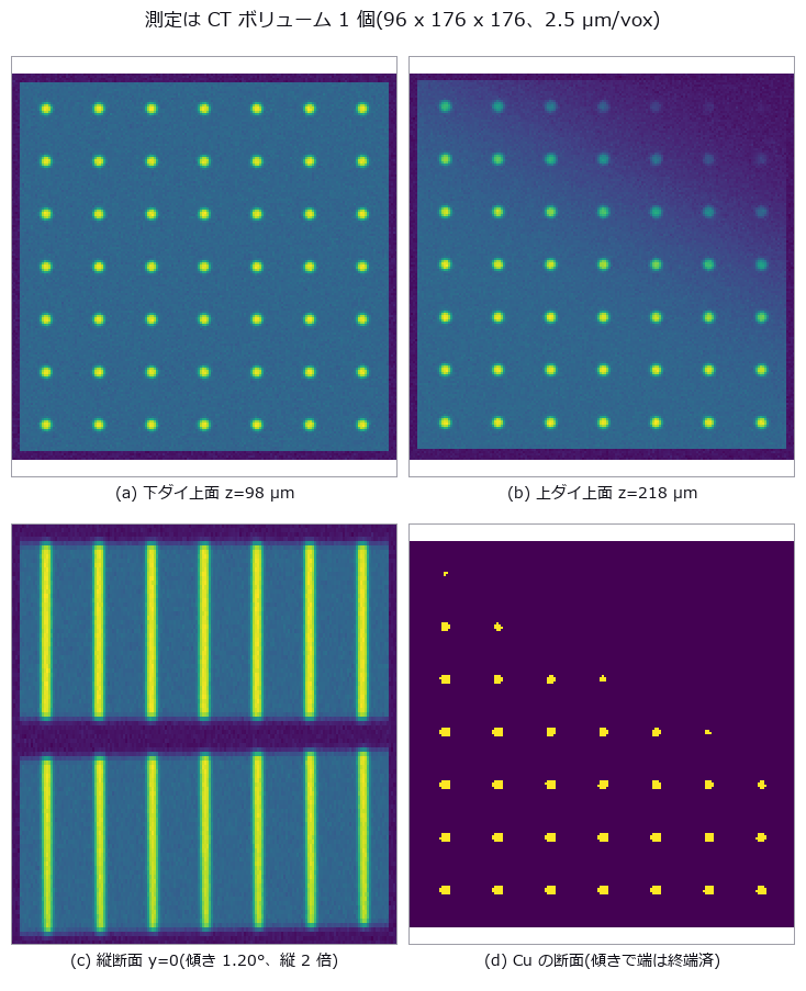
↑ Die tilt and TSV overlay from one CT — tilt fakes rotation too ―― Two stacked dies carry a 7x7 TSV lattice with a planted overlay of (+0.800, -0.450) um, +0.01500 deg of rotation and a die tilt of (1.20, 0.70) deg; a single CT volume is the whole measurement. Comparing the top-surface via openings directly misses by 2.419 um — 2.4x the +-1.0 um spec, and larger than the 0.918 um real overlay. The bias matches the closed form ‘die thickness x lateral part of the top-surface normal’ to a ratio of 0.996 / 0.999, and re-projecting each via down its own fitted axis recovers the truth to 0.0023 um. The prediction that failed: tilt fakes rotation as well as translation, through the sin(alpha)sin(beta) shear of Rx Ry — predicted +0.00733 deg against +0.00696 deg measured as the difference from the zero-tilt control. Axis correction does not remove it; only de-projecting with the measured tilt does. The cliff lands at 0.492 deg measured against 0.491 deg predicted.

↑ The measurement ―― 雲ごと 2.42 µm ずれるのが傾きの偽装。散らばりの広がりは測定精度。 (figure labels are in Japanese; the numbers are the same)
py -3.11 examples/poc_die_tilt_tsv_overlay.py
Source: examples/poc_die_tilt_tsv_overlay.py
Ops used (notes): fit_line3 · procrustes_fit · vol_label
32. Dimensional Inspection of a Machined Part — Bias and Scatter as Two Numbers
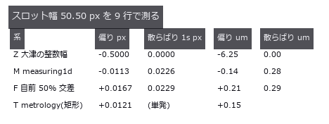
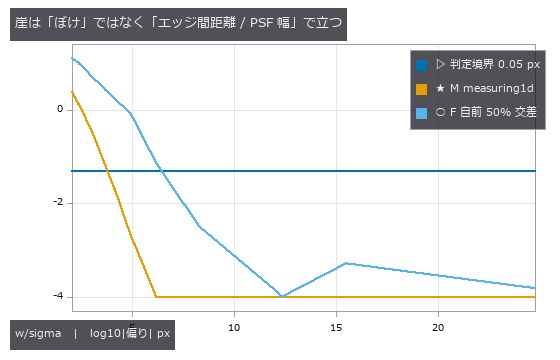
↑ Dimensional Inspection of a Machined Part — Bias and Scatter as Two Numbers ―― A part defined by a signed distance function (slot width 50.50 px, 1 px = 12.5 µm), imaged through a known PSF and noise and measured by four caliper systems. Otsu’s integer width (the null) has an RMS error of 0.464 px = 5.8 µm; the buried 1-D measuring implementation is biased by -0.0113 px = -0.14 µm, 41x better. Once the edge spacing drops below 3.09 PSF widths the width comes out systematically large, and the API keeps returning success.
| [](https://raw.githubusercontent.com/furuse-kazufumi/fullseye/master/docs/articles/assets/poc/poc_dimensional_inspection/02_blur_cliff.png) |
| *↑ The measurement ―― 偏りはどちらも正(対が互いを押し広げる)。符号が一定なので繰り返し測っても消えない。下端 -4 は表示の打ち切り( | 偏り | < 1e-4 px)。 (figure labels are in Japanese; the numbers are the same)* |
py -3.11 examples/poc_dimensional_inspection.py
Source: examples/poc_dimensional_inspection.py
Ops used (notes): add_metrology_object_circle_measure · add_metrology_object_ellipse_measure · add_metrology_object_generic · add_metrology_object_line_measure · add_metrology_object_rectangle2_measure · align_metrology_model · apply_metrology_model · create_metrology_model · edge_points · ellipse · fuzzy_measure_pairing · gen_measure_arc · gen_measure_rectangle2 · m1_measure_pairs · m1_measure_pos · measure_pairs · measure_pos · otsu · translate_measure
33. Fibre Orientation Distribution — Angles Repeat Every 180 Degrees, and a Naive Mean Is 90 Degrees Off
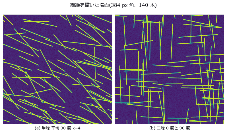
↑ Fibre Orientation Distribution — Angles Repeat Every 180 Degrees, and a Naive Mean Is 90 Degrees Off ―― Orientation of 140 fibres drawn from a von Mises distribution, read with a structure tensor. For a true mean of 177.9 degrees the arithmetic mean reports 105.55 degrees (-72.33), while the doubled-angle circular mean is off by +0.17 degrees — with not one bit of the image or the measurement changed. Weighting every pixel equally drops the orientation index by -31.3 %.
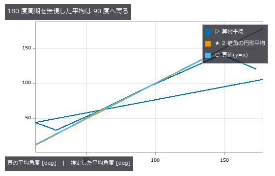
↑ The measurement (figure labels are in Japanese; the numbers are the same)
py -3.11 examples/poc_fiber_orientation.py
Source: examples/poc_fiber_orientation.py
Ops used (notes): coherence · dc_structure_texture · moment_axes · principal_moments · smooth_funct_1d_gauss · sobel_amp · sobel_dir
34. Gear Tooth Metrology — Eccentricity Is Order 1, Teeth Are Order z
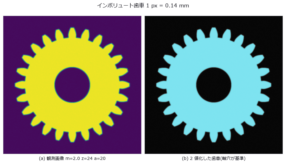
↑ Gear Tooth Metrology — Eccentricity Is Order 1, Teeth Are Order z ―― Eccentricity and tooth profile read from a gear drawn with the closed-form involute. The null’s least-squares circle has a diameter of 47.278 mm, which is neither the pitch (48), tip (52) nor root (43) circle. One missing tooth turns an eccentricity of 0.050 mm into 0.1285 mm (+157 %); the traditional method of one sample per tooth returns 0.0501 mm (+0.2 %).
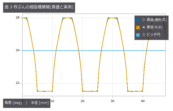
↑ The measurement (figure labels are in Japanese; the numbers are the same)
py -3.11 examples/poc_gear_tooth_metrology.py
Source: examples/poc_gear_tooth_metrology.py
Ops used (notes): blob_boundaries · blob_features · blob_label · blob_overlay · blob_region · blob_select_largest · gauss_filter · polar_trans_image · spectrum · threshold
35. How Accurately a White-Light Interferometer Measures a Nanometre Step
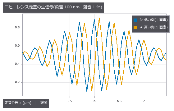
↑ How Accurately a White-Light Interferometer Measures a Nanometre Step ―― A synthesised coherence-scanning stack with steps of 50 to 500 nm measured back. At 1 % noise the bias stays within 2.4 nm and the standard deviation within 14.1 nm, almost independent of step height. The null (envelope’s maximum sample) errs by exactly half the scan step, and at 0.14 µm, just inside the Nyquist ceiling of 0.15 µm, the noise-free error is already +14.1 nm.
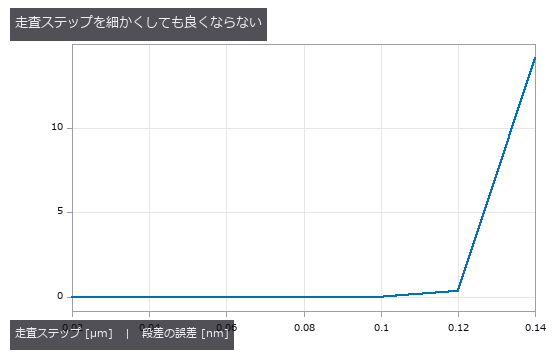
↑ The measurement ―― 0.02〜0.12 µm は 0.05 nm 以内で平ら。Nyquist 上限 0.15 µm の手前 0.14 µm で崖。 (figure labels are in Japanese; the numbers are the same)
py -3.11 examples/poc_interferometry_step.py
Source: examples/poc_interferometry_step.py
Ops used (notes): csi_design · csi_height_map · csi_stack_simulate · decode_fringe · gaussian · synthesize_fringes
36. Metallographic Grain Size — The Planimetric and Intercept Methods Fall Off Different Cliffs

↑ Metallographic Grain Size — The Planimetric and Intercept Methods Fall Off Different Cliffs ―― Grains are synthesized as a 2-D Voronoi tessellation with 2-px boundaries, then etching unevenness, noise and boundary gaps are added; ASTM E112 grain size G is measured by the planimetric method (Otsu + connected components) and the lineal-intercept method (local threshold + test lines in 4 directions). The planimetric method survives noise alone (-0.02) and etching unevenness alone (-0.40) but dies under both (+3.82), and loses one G step at 7.2 % boundary gaps; the intercept method holds to 40.7 % — the predicted 29.3 % was wrong because only 0.76 f of the boundary actually disappears in the mask. A duplex structure gives a whole-field G of 7.82 that matches neither the fine (9.01) nor the coarse (6.15) population; only 4 of 64 tiles fall within ±0.5 of it.

↑ The measurement (figure labels are in Japanese; the numbers are the same)
py -3.11 examples/poc_metal_grain_size.py
Source: examples/poc_metal_grain_size.py
Ops used (notes): bin_threshold · blob_features · blob_label · blob_overlay · bothat · dyn_threshold · gray_bothat · hx_close_edges · invert_image · otsu · threshold
37. Why the Seafloor Smiles — A Wrong Sound-Speed Profile Breaks Only the Outer Beams
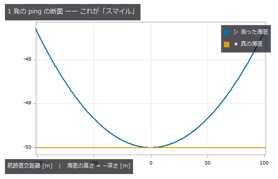
↑ Why the Seafloor Smiles — A Wrong Sound-Speed Profile Breaks Only the Outer Beams ―― Multibeam echosounding: get the water-column sound-speed profile wrong and a flat seafloor curls up (the classic smile / frown). Only the outer beams break — nadir is almost untouched, which is exactly the part the field checks with a bar check. The ground truth is planted here: a perfectly horizontal bottom at 50.0 m, sound speed 1520 to 1480 m/s (gradient -0.800 /s), 141 beams over +/-70 degrees, and the verdict comes from a real standard, IHO S-44 Order 1a (TVU at 50 m = 0.8201 m). The cliff was predicted twice before measuring: a rough expansion, dz = (g D^2 / 2 c0) tan^2(theta), gives 48.15 degrees, and the exact closed form (rays are circular arcs inside a constant-gradient layer) gives 48.68. The measurement with echo detection disabled lands on 48.68 — the exact form is right to 2.0e-11 m, while the expansion misses by 0.53 degrees (within 3.0 % out to 45 degrees, 19.4 % high at 70). One prediction was wrong: echo detection was expected to be a negligible floor, but the full-chain cliff is 47.95 degrees, 0.73 degrees earlier. At 70 degrees the illuminated strip stretches the echo to 21396 us (171 times the nadir value) and skews it, pulling the amplitude peak 0.725 m shallow — which is why real systems switch to phase detection on the outer beams. Controls separate the culprit: refraction alone is -2.6974 m, angle estimation contributes 0.000000 m and echo detection -0.2221 m. The textbook footprint formula is only 34 % of the truth at 70 degrees (cos^2 gives 8.21 m against a measured 24.14 m) because a steered array widens its beam as 1/cos(theta), so the correct exponent is three (cos^3 is off by -0.6 %). Discretisation alone can breach the standard: treating each cast layer as iso-velocity puts +1.2994 m on a 65-degree beam with two layers, converging first order to +0.0785 m with 32. The only check available without truth is the overlap between adjacent lines: 2.697 m of disagreement at the edge (3.3 times TVU) but exactly 0.0000 m in the middle of the overlap, where both lines use the same beam angle and the errors cancel — so it is invisible unless the full swath edge is compared. With upward refraction the outer beams never reach bottom: nothing is recorded rather than recorded wrongly (critical angle predicted at 73.90 degrees, bracketed by the last beam that arrives at 73.0 and the first that does not at 74.0). Across a 200-case grid of 25 sound-speed differences and 8 depths, 78.0 % of +/-65-degree swaths fail Order 1a at the edge. Finally, a one-way documentation hole was closed on the way: the vector-form refract only told callers to loop one ray at a time, never mentioning that refract_rays already returns a per-ray TIR mask.
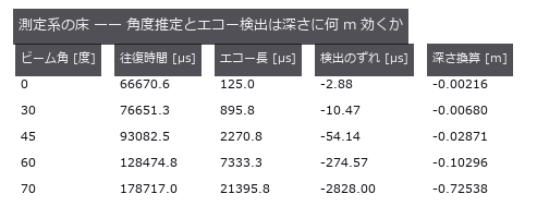
↑ The measurement ―― エコーは beamform_delay_sum の角度応答 × Lambert 後方散乱で海底の帯を足し上げて合成。find_peaks + peak_subbin で検出。 (figure labels are in Japanese; the numbers are the same)
py -3.11 examples/poc_multibeam_bathymetry.py
Source: examples/poc_multibeam_bathymetry.py
Ops used (notes): beamform_delay_sum · beamform_doa · dem_slope · find_peaks · interp_scattered · peak_subbin · snell_angle
38. Particle Size Distribution From Images — Merging and Edge Cuts Pull Opposite Ways and Cancel
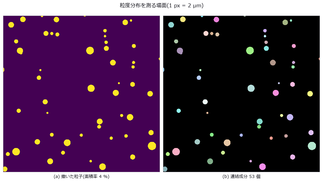
↑ Particle Size Distribution From Images — Merging and Edge Cuts Pull Opposite Ways and Cancel ―― D10 / D50 / D90 from a synthetic scatter of particles, with merges (pulling large) and edge cuts (pulling small) counted separately. At an area fraction of 13.8 % the D50 error is +0.55 % — because 28 merges and 19 edge cuts happen to balance. Number- and area-weighting give D50 values of 26.9 and 44.7 µm (1.66x) from the same blobs.
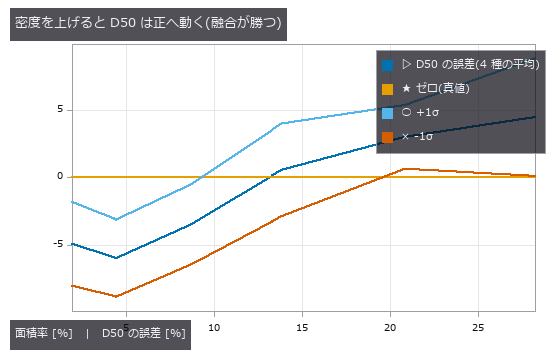
↑ The measurement ―― 薄いところで 0 なのは正確だから。濃いところで 0 をまたぐのは融合と縁切れが釣り合っただけ。 (figure labels are in Japanese; the numbers are the same)
py -3.11 examples/poc_particle_sizing.py
Source: examples/poc_particle_sizing.py
Ops used (notes): blob_features · blob_label · blob_overlay · blob_region · blob_select · circularity · distance_transform
39. Stress by Photoelasticity — Unwrapping Fails First at the Isotropic Point
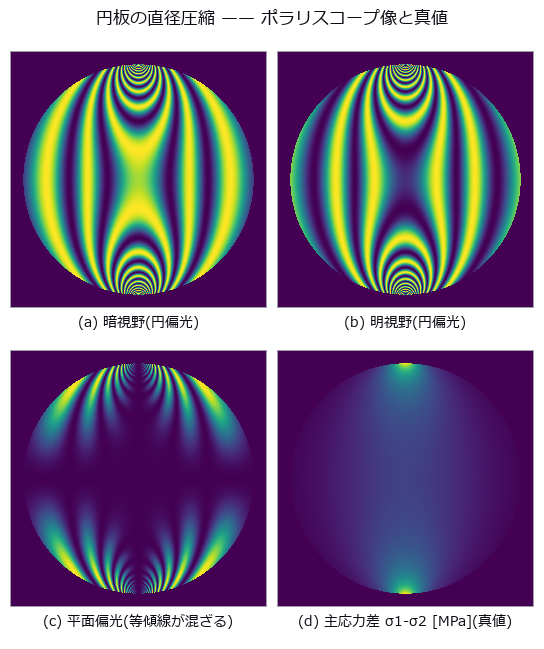
↑ Stress by Photoelasticity — Unwrapping Fails First at the Isotropic Point ―― The closed-form stress field of a diametrally loaded disc (4.2441 MPa at the centre, fringe order 2.380) turned into polariscope images by the Mueller-matrix ops and read back to stress. The op-built polariscope matches the textbook formula to 2.2e-16 across 125 cases. Phase wraps in the 84.2 % of pixels above fringe order 0.5, and unwrapping breaks first not where stress is highest but at the isotropic point, where modulation vanishes.
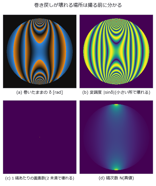
↑ The measurement ―― 左下 2 枚が「壊れる予報」。どちらもマスクで外せる。 (figure labels are in Japanese; the numbers are the same)
py -3.11 examples/poc_photoelasticity.py
Source: examples/poc_photoelasticity.py
Ops used (notes): mueller_apply · mueller_element · unwrap_phase_2d
40. Measuring Rail with a Chord — At the Wavelengths Where the Transfer Function Is Zero, Any Amplitude Reads Zero

| *↑ Measuring Rail with a Chord — At the Wavelengths Where the Transfer Function Is Zero, Any Amplitude Reads Zero ―― Reading track irregularity with a chord (versine) — the distance from the mid-point to a chord drawn between two points, still the working method in track recording and in acceptance of rail re-profiling. The null baseline, reading the versine directly as height, ranges from 0.0 % to 200.0 % of the truth depending on wavelength: one and the same 10 m chord reads lambda=10 m at +100 %, lambda=1.5 m at +50 %, lambda=30 m at -50 %, and lambda=5.0 / 2.5 / 1.0 m at -100 %. Over-reading and under-reading happen at once, so no single correction factor repairs it. The blind spots are exact geometry: | H(lambda) | = | 1 - cos(pi L / lambda) | is exactly zero at lambda = L/(2n) and doubles at lambda = L/(2n+1). Across ten wavelengths and two chords, twenty cases, prediction and measurement differ by at most 0.00000, and a 0.600 mm undulation at lambda=5.00 m gives a versine whose largest absolute value over 200 m is 0.00000 mm. Sorting into third-octave wavelength bands does not remove it (the ratio spans 0.00041 to 2.000, a factor of 4924), and the operator’s total_power earned its place here: the band sum is only 0.519 of the sum over all FFT bins, and the missing 48 % is the 30 m irregularity sitting below f_min — invisible if only the bands are read. Dividing by | H | to invert diverges to 6.9e7 mm at the blind wavelengths, and regularising it makes three wavelengths quietly report ‘no irregularity’. Two chords (10 m and 6 m) recover eight of the ten wavelengths to within 0.1 %, but the shared blind spot is not a point: it is the comb lambda = 1.000/k. One prediction was wrong — the planted lambda=0.100 m also survived, and it turned out to be the k=10 tooth. The relative spacing of the comb equals lambda itself, so it thickens toward short wavelengths: the corrugation band 0.03-0.30 m alone holds 30 blind wavelengths. At the 0.25 m sampling of a recording car, a 30 mm corrugation reappears as a 0.750 m undulation of 0.0528 mm, nine times the 0.00584 mm floor of a control with the short waves switched off. An asymmetric chord (3.7 m and 6.3 m arms) removes the long-wave blind spots, but | H | = 0 requires a/lambda and b/lambda to be integers together, so the blind spots move to lambda = gcd(a, b)/k = 0.100 m: the chord built to measure corrugation is blind inside the corrugation band.* |

↑ The measurement (figure labels are in Japanese; the numbers are the same)
py -3.11 examples/poc_rail_corrugation.py
Source: examples/poc_rail_corrugation.py
Ops used (notes): octave_bands · octave_spectrum
41. Counting and Measuring Real Coins — A Correct Answer Is Not a Safe One
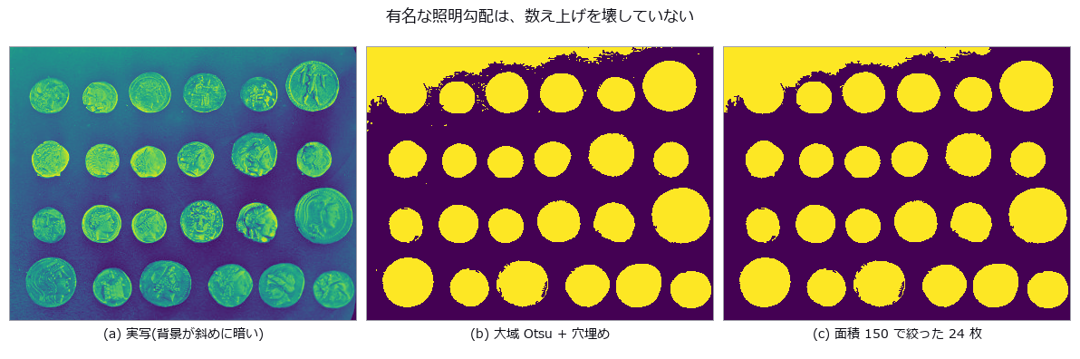
↑ Counting and Measuring Real Coins — A Correct Answer Is Not a Safe One ―― The real photograph famous for ‘a global threshold cannot work here, the lighting falls away across the frame’ (scikit-image coins). The background does slope, 0.427 to 0.161 down the rows and 0.331 to 0.059 across the columns — and yet a plain global Otsu with hole filling and an area floor of 150 lands exactly on the true 24. The truth is fixed by three independent paths agreeing (an area plateau spanning 50 to 800, a Hough circle search with the radii stated explicitly, and Sobel plus hole filling) and then checked one-to-one, each circle falling inside exactly one component. The margin, however, is 0.05: adding a little more of the same slope drops the count to 22. A correct answer is not evidence of a safe one. At +0.30 the median area moves by only -0.27 % while the worst single coin moves -24.20 %, and the drift correlates with row position at r = -0.90 — true area does not depend on where a coin sits, so that correlation is error, entire. Flattening with gray_tophat keeps the count but shrinks the median area to 0.29x, and the raw component count differs by 30 % between 4- and 8-connectivity.
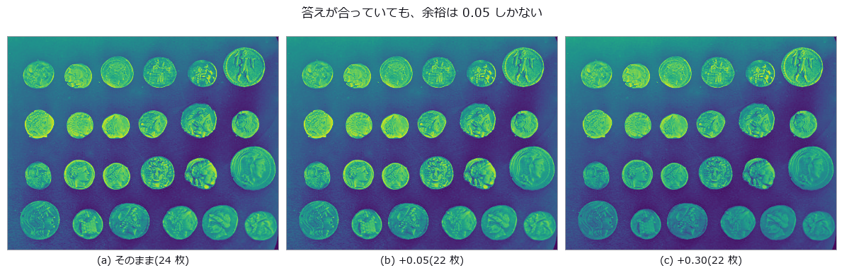
↑ The measurement ―― 見た目はほとんど変わらないのに 2 枚落ちる。 (figure labels are in Japanese; the numbers are the same)
py -3.11 examples/poc_real_coin_metrology.py
Source: examples/poc_real_coin_metrology.py
Ops used (notes): blob_count · blob_features · blob_label · canny · circularity · fill_holes · gray_tophat · hough_circle_trans · otsu · sobel_amp
42. Pitch, Flank Angle and Pitch Diameter From a Thread Silhouette — Tilt Shows Up With Opposite Signs on the Two Flanks
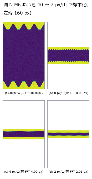
↑ Pitch, Flank Angle and Pitch Diameter From a Thread Silhouette — Tilt Shows Up With Opposite Signs on the Two Flanks ―― An M6-like silhouette drawn from the ISO 68-1 basic triangle in closed form (1 px = 25 µm). An FFT of the binarised column widths reports half the true pitch, 20 px, because the two profiles are offset by P/2 and their sum is constant. Tilting the axis by 3 degrees splits the flank angles into 33.18 / 26.74 degrees: their half-sum 29.81 is the true flank angle and their half-difference 3.19 estimates the tilt. Pitch measured on one flank drifts at first order (+3.28 / -2.79 %) while the crest spacing drifts at second order (-0.12 %); undoing the tilt leaves P -0.009 % and d2 +0.033 %.
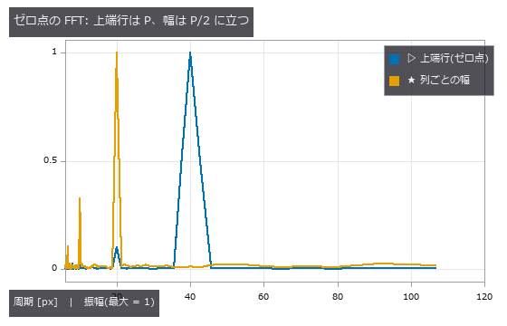
↑ The measurement ―― 幅の系列は上下輪郭(P/2 ずれ)の和なので基本波が消える。 (figure labels are in Japanese; the numbers are the same)
py -3.11 examples/poc_screw_thread_metrology.py
Source: examples/poc_screw_thread_metrology.py
Ops used (notes): fit_line_contours · gen_measure_rectangle2 · hx_split_contours · measure_pos · threshold · threshold_sub_pix · xg_regress_contours
43. Stockpile Inventory — The Answer Is Fixed by the Ground Nobody Measured
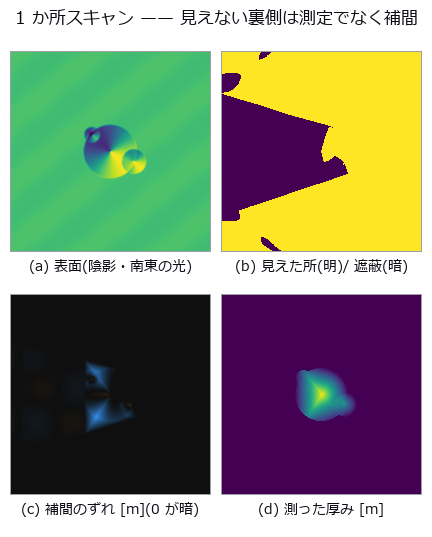
↑ Stockpile Inventory — The Answer Is Fixed by the Ground Nobody Measured ―― Stockpile inventory from a 3-D scan, for mining, aggregates and ports. The pile and the ground beneath it are written as separate formulas, and making the pile a sum of three cones at a 37 degree angle of repose closes the volume analytically at 3572.6089 m^3, matching a numerical integration at 0.025 m cells. The point is that the single number everyone quotes is fixed by a surface nobody measured: the ground under the pile. The first cliff is the assumed base, stated in closed form as dV = -A dh before measuring and matching to 0.0000 m^3 over seven offsets. The surprise is not the agreement but the size: 5 cm, which no survey would call an error, is 1.269 % of the inventory, or 72.5 t at a bulk density of 1.6 t/m^3 — three truckloads. The second cliff is occlusion. A cone is a ruled surface, so the visible fraction is arccos((H - h_s)/(D tan phi))/pi, matching to within 0.0201 over six geometries, and that residual halves with the cell size (0.0339, 0.0171, 0.0120 at 1.2, 0.6 and 0.4 m), which identifies it as discretisation rather than a wrong model. One prediction was wrong: interpolating across the occluded side was expected to under-estimate the volume, since a cone is concave and a chord passes below it, but the measurement is +17.20 %, an over-estimate. The far side is hidden all the way to the toe, so the triangulation connects the ridge not to the pile but to the ground beyond it, and a chord thrown 30 m past the ridge has a slope of 0.37 m/m that passes above the true 0.75 m/m slope. Then a cancellation trap: with the same single scan, using the true ground gives +17.20 % while the field practice of a horizontal base at the mean perimeter height gives +0.51 %. Nothing improved — the perimeter was lifted by the same interpolation, by +0.728 m, and the subtraction hides it; using only the perimeter points that were actually seen returns +12.05 %. A contaminated ruler applied to a contaminated object makes the error look like it went away. The same shape recurs with a berm of spoil at the toe: the outlier-resistant RANSAC fit reads worse (+2.48 %) than total least squares (+0.61 %), but RANSAC correctly rejected the berm and returned to the no-berm answer of +1.91 %, while TLS looked good because the berm’s lift happened to cancel the bias from the undulating ground. Averaging the perimeter cancels the ground’s tilt whenever the footprint is roughly symmetric — the flat control reads +0.01 % — so the remaining +1.79 % is entirely undulation, and fitting a tilted plane makes it worse (+1.91 %): more freedom does not mean less bias. The rulers disagree on the winner, with the horizontal base slightly better on volume and the fitted plane six times better on the centroid (0.07 m against 0.42 m), which is the quantity a loading plan uses. And the two errors do not add: -0.70 % expected against +0.51 % measured, because the occlusion fill moves the perimeter that fixes the base. Finally, a real bug was found and fixed: dem_viewshed reported every cell above the observer’s eye as not visible — the apex of a cone on open flat ground read 0.0, none of the 1541 cells above eye level were visible, and the occluded fraction came out 0.8863 against a closed-form 0.5710. Line-of-sight samples rounded onto the target cell itself, occluding it against its own height; skipping those samples restores 1.0 at the apex and 0.5900 for the occluded fraction. The existing tests missed it because they only checked flat ground and what lies behind a wall, never whether the wall itself is visible.
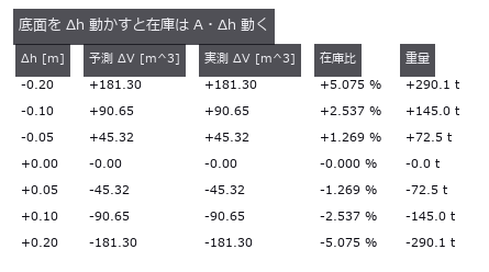
↑ The measurement ―― A = 906.5 m^2。閉形式は測る前に印字してある。 (figure labels are in Japanese; the numbers are the same)
py -3.11 examples/poc_stockpile_volume.py
Source: examples/poc_stockpile_volume.py
Ops used (notes): dem_hillshade · dem_slope · dem_viewshed · interp_scattered · moment_axes
44. Strain History in a Creep Test — Cumulative or Direct?
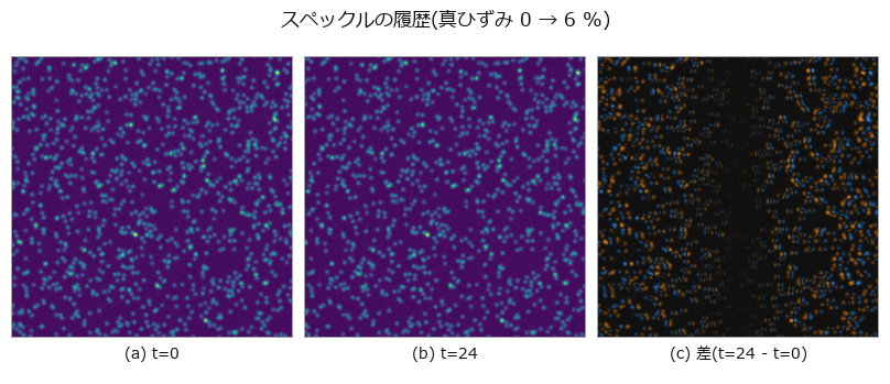
↑ Strain History in a Creep Test — Cumulative or Direct? ―― One hour of creep in 25 frames, with strain history from accumulating adjacent-frame displacements versus comparing each frame directly with the reference. At the end, cumulative errs by 61 µε and direct by 1878 µε — cumulative wins 31x and the textbook crossover in time never appears (it lives on the noise axis instead). Thinning from 24 to 4 steps worsens cumulative from -60 to -606 µε; what matters is the deformation per step, not the number of steps.
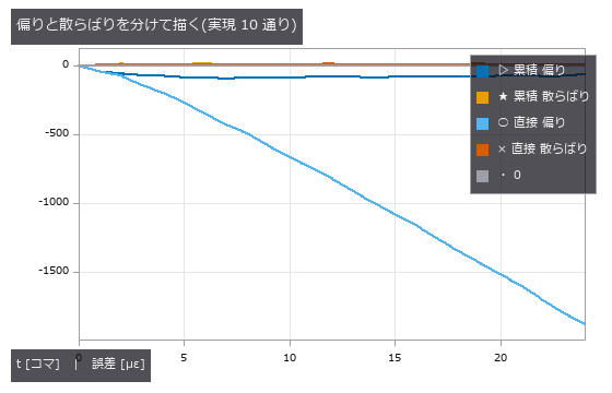
↑ The measurement ―― 直接の偏りだけが伸びる。累積は偏りも散らばりも頭打ちで、しかも散らばりより偏りのほうが大きい ——ランダムウォークではない。 (figure labels are in Japanese; the numbers are the same)
py -3.11 examples/poc_strain_history.py
Source: examples/poc_strain_history.py
Ops used (notes): moving_average_window · piv_cross_correlate · piv_error_stats · piv_multipass · piv_sample_at_windows · piv_synth_pair · poly_fit
45. How Far Sa / Sq / Sz Survive Sampling and Cutoff
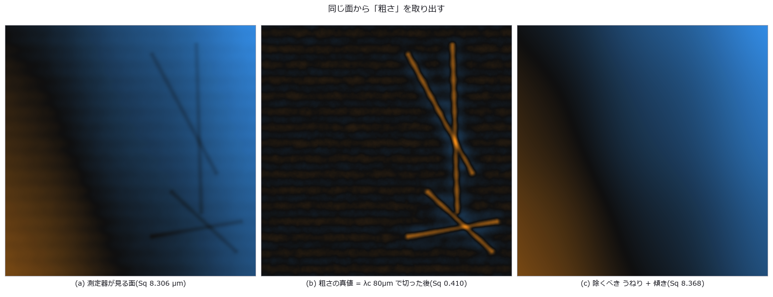
↑ How Far Sa / Sq / Sz Survive Sampling and Cutoff ―― A surface synthesised from a prescribed PSD (so the true Sq follows analytically from Parseval), with tilt, waviness, lay and scratches added before the roughness parameters are measured. Calling the raw rms ‘Sq’ overstates it 20x; removing only the plane still leaves 1.8x. At 8 µm sampling Sa is -3.5 % (pass) while Sz is -19.8 % (fail); Sz keeps growing with evaluation area and never plateaus, so there is no such thing as the true Sz.
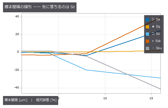
↑ The measurement ―― dx=8 µm では Sa が ±5 % 合格で Sz が不合格。同じデータでも見るパラメータで結論が反転する。 (figure labels are in Japanese; the numbers are the same)
py -3.11 examples/poc_surface_roughness.py
Source: examples/poc_surface_roughness.py
Ops used (notes): profile_params · surface_filter · surface_form_remove · surface_params · surface_psd · surface_synth_psd
The Medical and Biological Wing — The Count Is Right and the Contents Are Wrong
Counting cells, reading a nucleus’s DNA content, measuring vessel branching, tracking a wound’s area: all of these tend to be reported as one number, and there are situations in which that number is right anyway. Cell counting where over- and under-segmentation balance to a +0.3-cell bias; ploidy classification that survives a forgotten background subtraction; a calibration that returns the most stable and most wrong healing constant.
The four exhibits carry ground truth that a label image alone cannot hold — which cells overlap which, area and DNA content varying independently, a tree that satisfies the branching law exactly. Each docstring warns that calling a label image ‘the truth’ on real data erases the very thing being tested.
The thing to watch for is a method that appears to improve while the quantity it measures quietly swaps: the area classifier gets better with more blur because ‘area’ is leaking DNA content. Unless the reason for every improvement is traced, this kind of lie gets carried home as a result.
46. Trabecular Thickness, Separation and Bone Volume Fraction — The Plate Model and the Direct Method Disagree on the Same Image
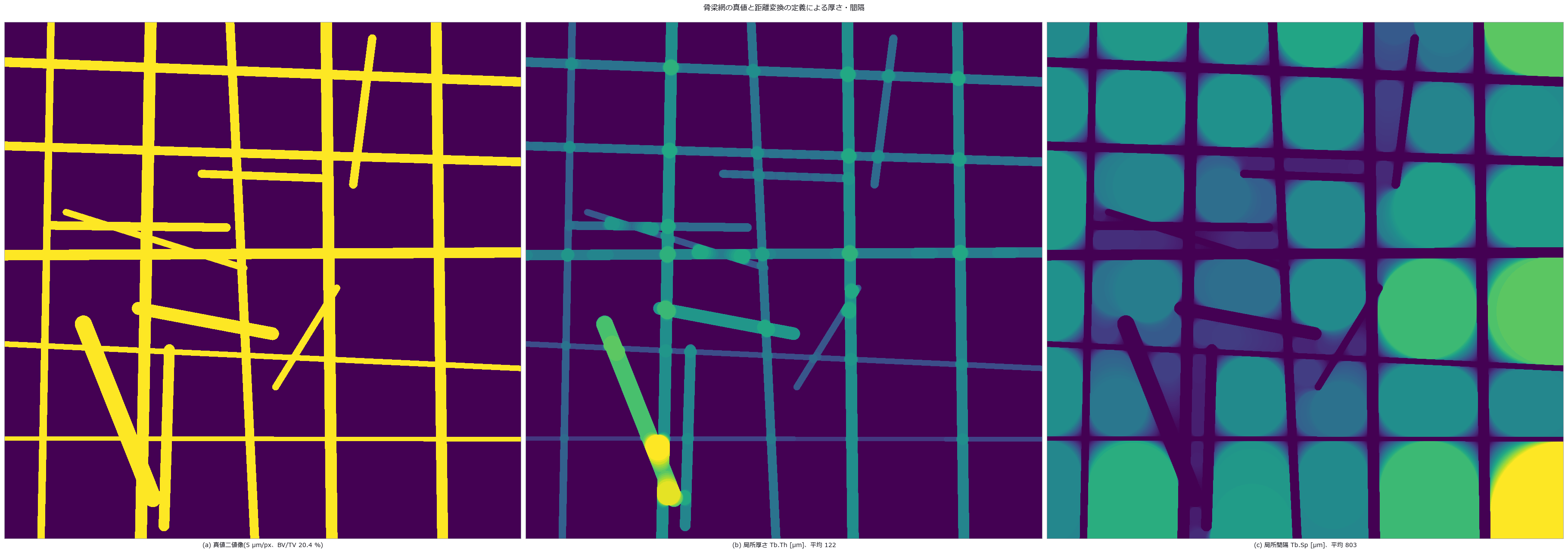
↑ Trabecular Thickness, Separation and Bone Volume Fraction — The Plate Model and the Direct Method Disagree on the Same Image ―― A 2-D trabecular network drawn in closed form as a set of segments (median width 120 µm), observed through partial-volume blur, CT noise and a cupping bias. There is more than one ground truth: the length-weighted mean width is 104.8 µm, the largest-inscribed-circle definition gives 121.6 µm and the plate model 118.4 µm — the choice of truth moves the answer by 9–16 % before any threshold does. The resolution cliff hits the distribution, not the mean (overlap with truth 0.83 → 0.09 at 60 µm pixels; the mean survives because quantisation at -29.5 % and Otsu thickening at +27.1 % cancel). Noise breaks from two sides, speckles from σ 0.10 and gaps from σ 0.15, and an area opening removes only the speckles.
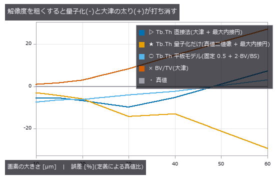
↑ The measurement ―― Tb.Th の平均は 2 px/骨梁でも持つが、BV/TV と分布は壊れている。 (figure labels are in Japanese; the numbers are the same)
py -3.11 examples/poc_bone_trabecular_thickness.py
Source: examples/poc_bone_trabecular_thickness.py
Ops used (notes): blob_distance · blob_features · blob_label · dc_retinex · dist_transform · gaussian · get_region_thickness · opening_circle · otsu · sk_area_opening · threshold
47. Counting Overlapping Cells — Count, Over-Segmentation and Under-Segmentation as Three Numbers
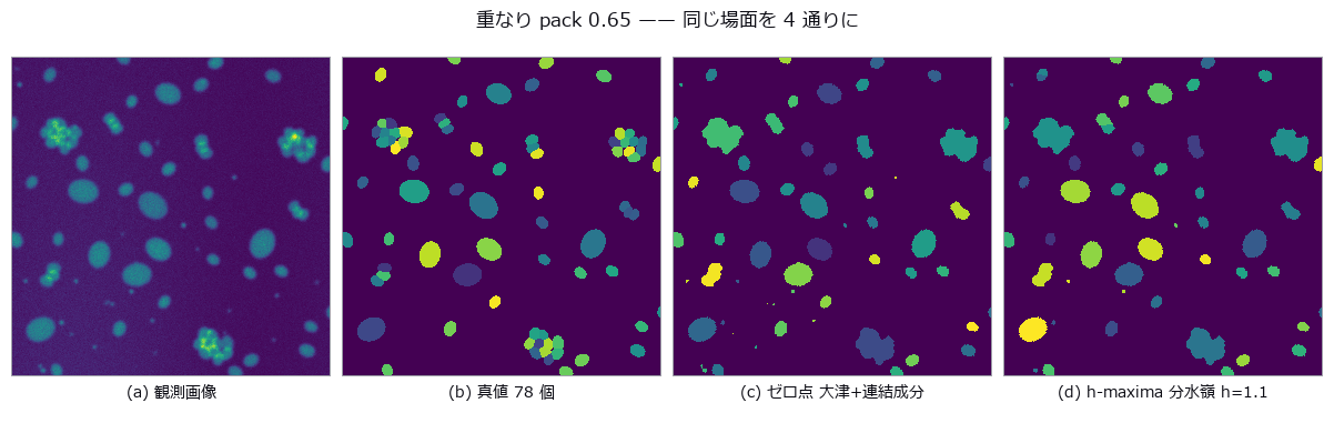
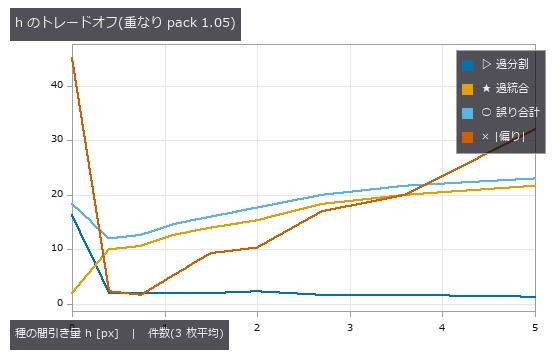
↑ Counting Overlapping Cells — Count, Over-Segmentation and Under-Segmentation as Three Numbers ―― Synthetic overlapping cells with the count, over-segmentation and under-segmentation tallied separately. In the densest condition the null misses 25 of 78 cells, every one of them an under-segmentation. Sweeping the seed suppression finds a balance point where the count bias is +0.3 cells while 13.3 segmentation errors remain; report the count alone and it passes as the best setting.
| [](https://raw.githubusercontent.com/furuse-kazufumi/fullseye/master/docs/articles/assets/poc/poc_cell_counting/02_h_tradeoff.png) |
| *↑ The measurement ―― 誤り合計の谷と | 偏り | の谷は同じ場所に来ない。どちらを最適と呼ぶかで答えが変わる。 (figure labels are in Japanese; the numbers are the same)* |
py -3.11 examples/poc_cell_counting.py
Source: examples/poc_cell_counting.py
Ops used (notes): circularity · distance_transform · fill_holes · gauss_filter · sk_otsu · vol_distance_transform · vol_label · vol_local_maxima · vol_watershed · xsk2_h_maxima
48. Colocalization lies under bleed-through — Pearson and Manders break in different places
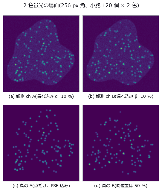
↑ Colocalization lies under bleed-through — Pearson and Manders break in different places ―― Two channels of vesicle-like puncta are scattered over a synthetic cell body, with 0 / 25 / 50 / 100 % of the B puncta placed exactly on A puncta so the true colocalization is known. After the bleed-through matrix [[1, α], [β, 1]], cytoplasm, PSF and photon noise, two unrelated channels give Pearson r=0.203 and Otsu-Manders M1=0.133 at α=β=10 %. Estimating α=0.0996 (truth 0.10) from single-stain controls and unmixing linearly restores r to 0.007, but Manders stays at 0.705 even for 100 % (the Gaussian tails below the Otsu threshold are lost; closed-form prediction 0.756). Pearson crosses 0.5 at symmetric α=0.282 (predicted 2−√3=0.268); blur only breaks Manders, with a step at σ=2.5 px where Otsu’s foreground jumps from puncta to the whole cell. The Costes shuffle test calls pure bleed-through ‘significant’ at p=0.000.
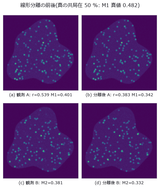
↑ The measurement (figure labels are in Japanese; the numbers are the same)
py -3.11 examples/poc_colocalization_crosstalk.py
Source: examples/poc_colocalization_crosstalk.py
Ops used (notes): gauss_image · mat_lstsq · mat_solve · noise_sigma · otsu · photon_sample · reg_erode · stat_correlation
49. MRI Bias Field and Tissue Area — Grey and White Matter Fail in Opposite Directions, and the Sum Hides It
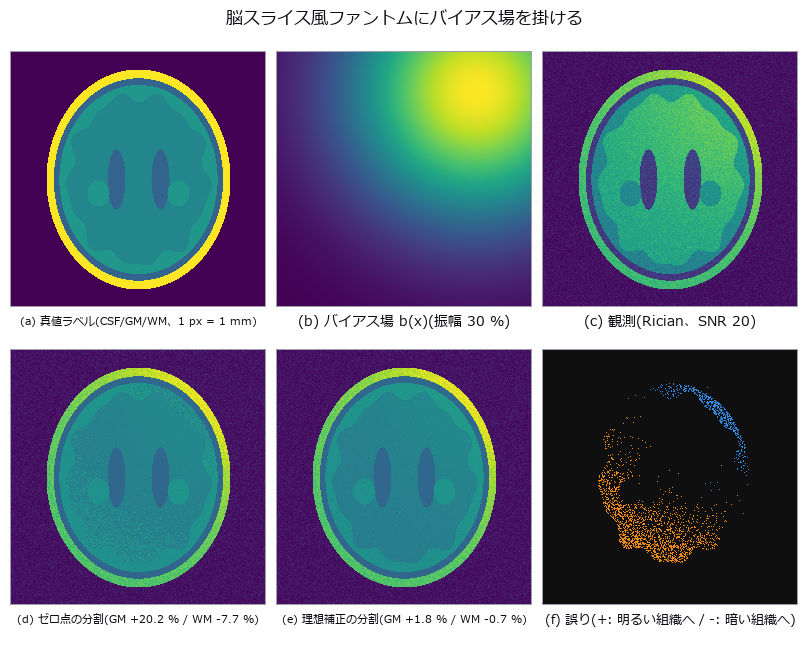
↑ MRI Bias Field and Tissue Area — Grey and White Matter Fail in Opposite Directions, and the Sum Hides It ―― A brain-slice phantom of elliptical shells (skull / CSF / wrinkled cortex / WM, areas known from geometry) is multiplied by a surface-coil bias field and Rician noise, and the three tissue areas are measured with global three-class Otsu (xsk2_multiotsu). At 30 % amplitude GM is +20.2 % and WM -7.7 % while GM+WM is +0.0 % — the sum hides the error — and removing the noise flips the sign (GM -11.8 %). The geometric cliff prediction was 30 %; the measured cliff is 17.5 %. Naively smoothing log I damages a field-free image by GM +81.8 %; iterating on the segmentation residual (Wells-type) holds +1.8 % even at 40 %. Every corrector fails once the field is as fine as 4 px, and at SNR 15 GM is +8.5 % even without a field (WM is 2.6× larger, so the error lands on the smaller tissue).
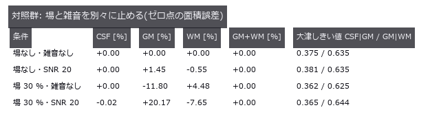
↑ The measurement ―― 雑音だけでは壊れず、場だけで GM と WM が逆向きに動く。 (figure labels are in Japanese; the numbers are the same)
py -3.11 examples/poc_mri_bias_field.py
Source: examples/poc_mri_bias_field.py
Ops used (notes): dc_homomorphic · eval_bspline_surface · eval_poly_surface · fit_bspline_surface · fit_poly_surface · overlay_labels · xsk2_multiotsu
50. Ploidy From Integrated Nuclear Intensity — Area Cannot Separate It
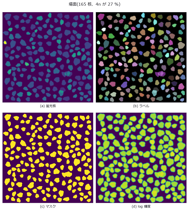
↑ Ploidy From Integrated Nuclear Intensity — Area Cannot Separate It ―― Fluorescent nuclei whose DNA content D and area A were drawn with independent spread, classified by area and by integrated intensity. Even the true area misclassifies 15.4 %; integrated intensity misclassifies 0 %. Forgetting to subtract background leaves the classification intact while the DNA index alone breaks from 2.115 to 1.702 (-20 %) — invisible if you only watch the classification.
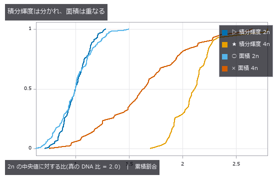
↑ The measurement ―― 累積分布。積分輝度の 4n は 2.1 付近に固まり、面積の 2 本は大きく重なる。 (figure labels are in Japanese; the numbers are the same)
py -3.11 examples/poc_nuclei_ploidy.py
Source: examples/poc_nuclei_ploidy.py
Ops used (notes): aperture_photometry · blob_features · blob_label · blob_overlay · gaussian · median · sg_gmm_segment · sk_otsu
51. Extracting a Vessel Network — Spurs, Overestimated Radii Near Branches, and a Fragile Exponent
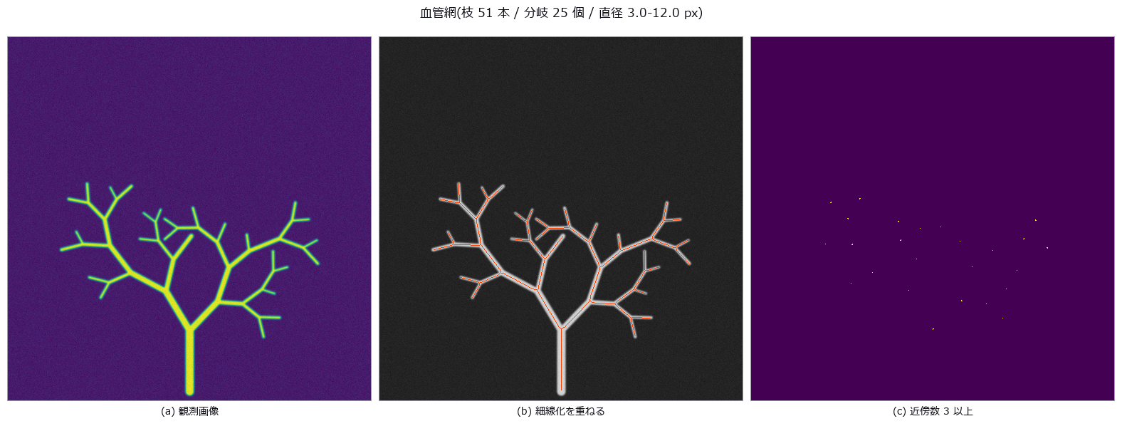
↑ Extracting a Vessel Network — Spurs, Overestimated Radii Near Branches, and a Fragile Exponent ―― A synthetic vessel tree obeying Murray’s law exactly, skeletonised and measured for branch points, radii and the exponent. Counting branch pixels directly gives 47 pixels for 25 branches; grouping them into connected components gives exactly 25. Spurs come not from the skeletonisation but from boundary roughness (spurious branches 0 → 72), and radii within 3 px of a branch are overestimated by +26.2 %.
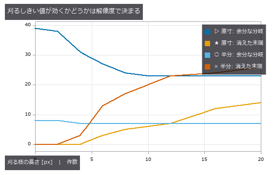
↑ The measurement (figure labels are in Japanese; the numbers are the same)
py -3.11 examples/poc_vessel_network.py
Source: examples/poc_vessel_network.py
Ops used (notes): blob_features · blob_label · distance_transform · gauss_filter · medial_axis_points · r2_split_skeleton_lines · sk_medial · skeleton · skeleton_branches3d · skeleton_endpoints3d · skeleton_junctions3d · skeleton_prune3d · skeletonize_vol · thinning · vol_distance_transform
52. Wound Area Over Time — Calibration Error Enters the Area Squared
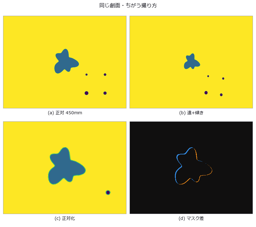
↑ Wound Area Over Time — Calibration Error Enters the Area Squared ―― A star-shaped wound on a millimetre plane (closed-form area), photographed day by day through a pinhole camera to estimate the healing constant k. A 4 % change in distance moves the area by 7.7 %; with the distance drifting 1.2 % per day the null reports k = 0.1424 against a true 0.1200 (+18.7 %). Its standard deviation, 0.0049, is smaller than the 0.0059 of recalibrating every time — the most stable and the most wrong answer.

↑ The measurement ―― ゼロ点の面積誤差。実測は閉形式の 2 乗則に乗り、線形近似からは外れる。 (figure labels are in Japanese; the numbers are the same)
py -3.11 examples/poc_wound_area_tracking.py
Source: examples/poc_wound_area_tracking.py
Ops used (notes): blob_features · blob_label · blob_select_largest · gaussian · warp_by_plane
The Astronomy and Environment Wing — Biased by Position, Flipped by the Definition of Truth
Stellar brightness and position, the solar limb, all-sky cloud cover, sea-ice concentration, crop cover, terrain, river stage. The subjects are far away and ground truth is normally out of reach. The eight exhibits here turn that around, placing their truth in closed forms and public data: celestial coordinates, the solid angle of a spherical cap, Eddington limb darkening, elevation tiles from the Geospatial Information Authority of Japan.
The shared finding is that the same object reads differently depending on where it is: the same cloud counts 1.45x more at the horizon than at the zenith; clouds of equal optical thickness are detected or not depending on their angular distance from the sun; the same reflection makes one detector read quietly low and another stop silently.
The other is that the definition of truth decides the conclusion. Counting thin ice as ‘ice’ or not sends the same estimate to -4.4 or +2.7 points; a cloud fraction reported without its horizon-mask angle can legitimately claim anything from 0.18 to 0.23. What you call the truth has to be written down before the instrument is.
53. All-Sky Cloud Cover — Counting Pixels Is Biased by Position
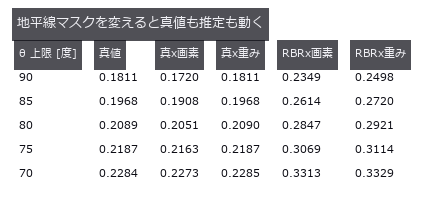
↑ All-Sky Cloud Cover — Counting Pixels Is Biased by Position ―― Spherical-cap clouds (closed-form solid angle) placed in an equidistant fisheye sky, with cloud fraction counted by pixel ratio and by solid-angle weight. The same cloud reads 0.00789 at the zenith and 0.01142 at 82 degrees (1.45x). Geometry alone errs by -5.02 %, detection alone by +37.95 %, and the naive count cancels them to +29.73 %.
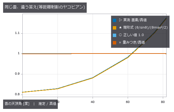
↑ The measurement ―― 画素数比は天頂で 0.81、地平線側で 1.17。重みを掛けると 1 に張り付く。 (figure labels are in Japanese; the numbers are the same)
py -3.11 examples/poc_allsky_cloud_cover.py
Source: examples/poc_allsky_cloud_cover.py
Ops used (notes): polar_trans_image
54. How Many Frames for What Photometric Precision?
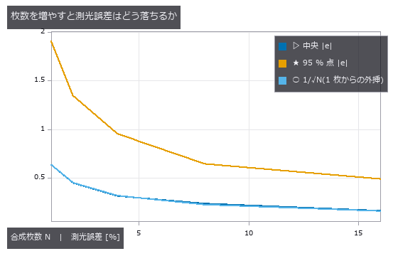
↑ How Many Frames for What Photometric Precision? ―― A star field placed to specification and stacked N deep, to see whether aperture-photometry error falls as 1/√N. From N = 1 to 16 the median error drops from 0.6350 % to 0.1616 %, within 4.6 % of theory in all eight cases. One cosmic ray pushes the plain mean to +5.89 % while κ-σ clipping holds +0.30 %; the rejection rate does not move, so ‘the rejection rate went up, therefore it worked’ is not an available argument.
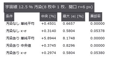
↑ The measurement ―― 単純平均だけが 5.9 % 残る。κ-σ は汚染なしと区別できないところまで戻すが、棄却率はほとんど動かない。 (figure labels are in Japanese; the numbers are the same)
py -3.11 examples/poc_astro_photometry.py
Source: examples/poc_astro_photometry.py
Ops used (notes): aperture_photometry · drizzle_resample · lucky_select · median · sigma_clip_stack · synth_frame_series · synth_starfield
55. Change detection under misregistration — false positives are edge bands, with a cliff

↑ Change detection under misregistration — false positives are edge bands, with a cliff ―― A two-date synthetic land surface (fields, roads, buildings, forest, lake) with planted changes (new buildings, clear-cut, lake expansion); date 2 is degraded by sub-pixel shift, small rotation and an illumination change, and the false-positive area of plain differencing is measured. False positives stay at the noise floor up to 0.3 px and jump at 0.5 px (matching the PSF-derived onset δ=τσ√2π/C=0.351 px), reaching 7175 px at 3 px. The edge-length × shift rule gives 0.78× at 3 px but cannot explain the cliff; the PSF+noise edge-ledger prediction is within 0.84–1.07×. Three registration paths (PIV, keypoints, LK) bring the residual down to 0.02–0.13 px, but the only phase-correlation path is 3-D and integer-valued (residual 0.72 px), and its 995 px of false positives lands on the shift-only sweep read at the same residual (915 px). Clear-cut recall is 0.33 even with perfect alignment; the illumination-only 17198 px vanish with radiometric normalisation while the 3497 px from shift do not.*

↑ The measurement ―― 0.35 px までゼロ、そこから立ち上がる。比例則は崖を説明しない。 (figure labels are in Japanese; the numbers are the same)
py -3.11 examples/poc_change_detection_misreg.py
Source: examples/poc_change_detection_misreg.py
Ops used (notes): affine_trans_image · histogram_match · match_phase_3d · opening_circle · piv_cross_correlate · piv_outlier_mask · procrustes_fit · threshold · voxel_iou
56. A 3-D Thermal Field from Sparse Sensors — The Grid’s Blind Spot Erases a Rack
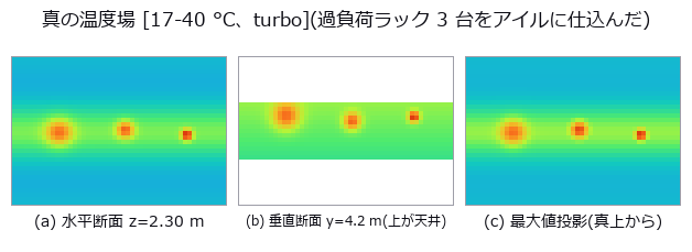
↑ A 3-D Thermal Field from Sparse Sensors — The Grid’s Blind Spot Erases a Rack ―― A temperature field for a 12 x 8.4 x 3.0 m server room is written as a formula, then reconstructed from a grid of temperature sensors to find three overloaded racks. The null baseline, the mean of all sensors spread over the whole room, gives an RMSE of 2.192 degrees and finds no hot spot at all; the best method, a thin-plate RBF, gives 0.214, ten times better. The cliff can be stated in closed form before measuring: on a grid of spacing d the point furthest from a peak is the cell centre at dsqrt(3)/2, so a Gaussian of width sigma is recovered at exp(-3d^2/8sigma^2) and halves at d* = 1.3596 sigma. Isolating the geometry, prediction and measurement differ by at most 1.2e-15. What failed was not the formula but the quantity a site can actually measure: the peak of a reconstructed field carries the background’s reconstruction error at the same place, so a naive measurement exceeds the prediction by up to +0.2598 and the cliff looks shallower than it is. The sigma=0.22 m rack is recovered at 0.000014 at d=1.20 m, effectively gone, yet naively appears to hold 0.1609 — what remains is the background error. The closed form is a floor, not a curve: at the same d=0.60 m, recovery jumps from 0.0615 at a cell centre to 1.0 directly above a sensor, so only the worst phase is usable for design. Random placement does not remove blind spots; it only reshuffles which rack falls into one. Measured, 6.17 % of random points exceed the grid’s worst distance against a Poisson prediction of 6.58 %. The grid never breaks its geometric lower bound while random placement broke it for two of the three racks: with the same sensor count, only one of them supports a guarantee. Swapping the interpolator moves the coefficient, not the exponent — all three slopes of log recovery against d^2 sit within 3.05 % of the predicted -3.0612 — but the prediction that the cliff position is method-independent was wrong: the thin-plate spline overshoots its own nodes by a factor of 1.372 and shifts the half-recovery spacing from 0.4777 to 0.6015 m, a 26 % move. The follow-up prediction, that an overshooting method raises the false peaks by the same factor, was also wrong: the nearest-neighbour floor is 0.975 degrees, 6.5 times the sensor noise, because a staircase approximation of a smooth background is itself a step. No method wins all three rulers at once, and at d=1.20 m linear interpolation falls outside the convex hull for 71.2 % of the evaluation points, silently becoming nearest-neighbour at the walls. The gap this PoC found has since been filled: fs.interp_scattered interpolates a field from scattered N-D points and returns the fraction of query points that fell outside the convex hull — the 71.2 % measured here is exactly the quantity that would otherwise turn silently into NaN or into another method under the first method’s name.*
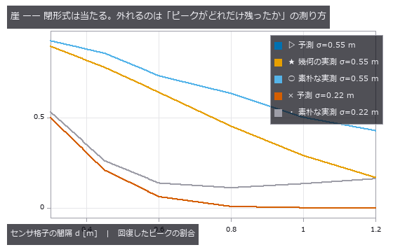
↑ The measurement ―― 幾何の実測は予測と最大 1.2e-15 しか違わない。素朴な実測が上に浮くぶんが背景の復元誤差。 (figure labels are in Japanese; the numbers are the same)
py -3.11 examples/poc_datacenter_thermal_field.py
Source: examples/poc_datacenter_thermal_field.py
Ops used (notes): interp_scattered · render_volume_projection · rmse · vol_local_maxima
57. Measuring Terrain — Slope, Flow and Insolation Against Closed Forms
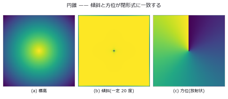
↑ Measuring Terrain — Slope, Flow and Insolation Against Closed Forms ―― Slope, curvature and sky-view factor checked against closed forms on a plane, a cone and a Gaussian hill. Halving the cell size cuts the hill’s curvature error by about four — a discretisation error, not a wrong formula. The sky-view factor takes 2.03 s on a 513×513 grid with 8 directions; before the rewrite it took 41.9 s, and the tests had only ever checked that it runs.
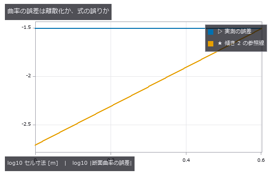
↑ The measurement ―― 参照線と平行 = 2 次収束 = 離散化の誤差。式が違えばセルを細かくしても誤差は下げ止まる。 (figure labels are in Japanese; the numbers are the same)
py -3.11 examples/poc_dem_terrain.py
Source: examples/poc_dem_terrain.py
Ops used (notes): dem_aspect · dem_curvature · dem_fill_sinks · dem_flow_accumulation · dem_hillshade · dem_sky_view_factor · dem_slope
58. Exoplanet transit from aperture photometry — depth and duration fail separately
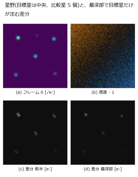
↑ Exoplanet transit from aperture photometry — depth and duration fail separately ―― A synthetic star field (240 frames) carries a 10 ppt limb-darkened transit on the target only, with transparency variation, sub-pixel drift, flat-field non-uniformity and photon noise injected from separate random streams; fullseye’s star_detect → frame_align → aperture_photometry extracts the light curve. The zero point (target aperture sum alone) breaks under clouds to a depth error of +72 ppt; the ratio to comparison stars gives -0.13 ppt / T14 -0.9 fr. Comparison-star choice moves the residual rms from 1.91 to 11.43 ppt (6.0x), and inverse-variance weights computed from raw variance are fooled by clouds into 1.52x worse than a plain sum. The small-aperture cliff at 1σ was not the predicted centroid error but the op’s aperture-mask staircase (supersample=8: a static star sits 1.69x above theory, 0.93x at 32). The SNR=5 detection limit is 1.48 ppt measured vs 1.45 ppt theory with a known ephemeris, 2.0 ppt blind, where the duration breaks before the depth. Drift 2 px and a 3 % flat are harmless alone (0.16 / 0.08 ppt) but multiply into a 0.94 ppt false depth, 2.97 ppt (30 % of truth) at 4 px.
[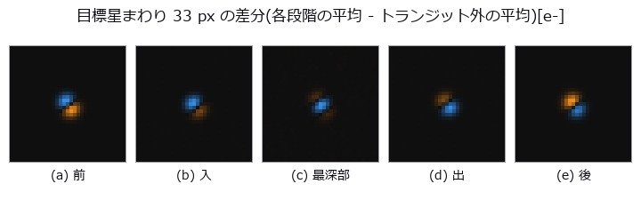](https://raw.githubusercontent.com/furuse-kazufumi/fullseye/master/docs/articles/assets/poc/poc_exoplanet_transit/02_frames_transit_phases.png)
↑ The measurement ―― 前/入/最深部/出/後の各段階で平均した画像からトランジット外の平均を引いた [e-]。4 倍拡大 (figure labels are in Japanese; the numbers are the same)
py -3.11 examples/poc_exoplanet_transit.py
Source: examples/poc_exoplanet_transit.py
Ops used (notes): aperture_photometry · frame_align · normalize · sigma_clip_stack · star_detect
59. Coordinates Go Wrong by Tens of Metres While Still Looking Plausible
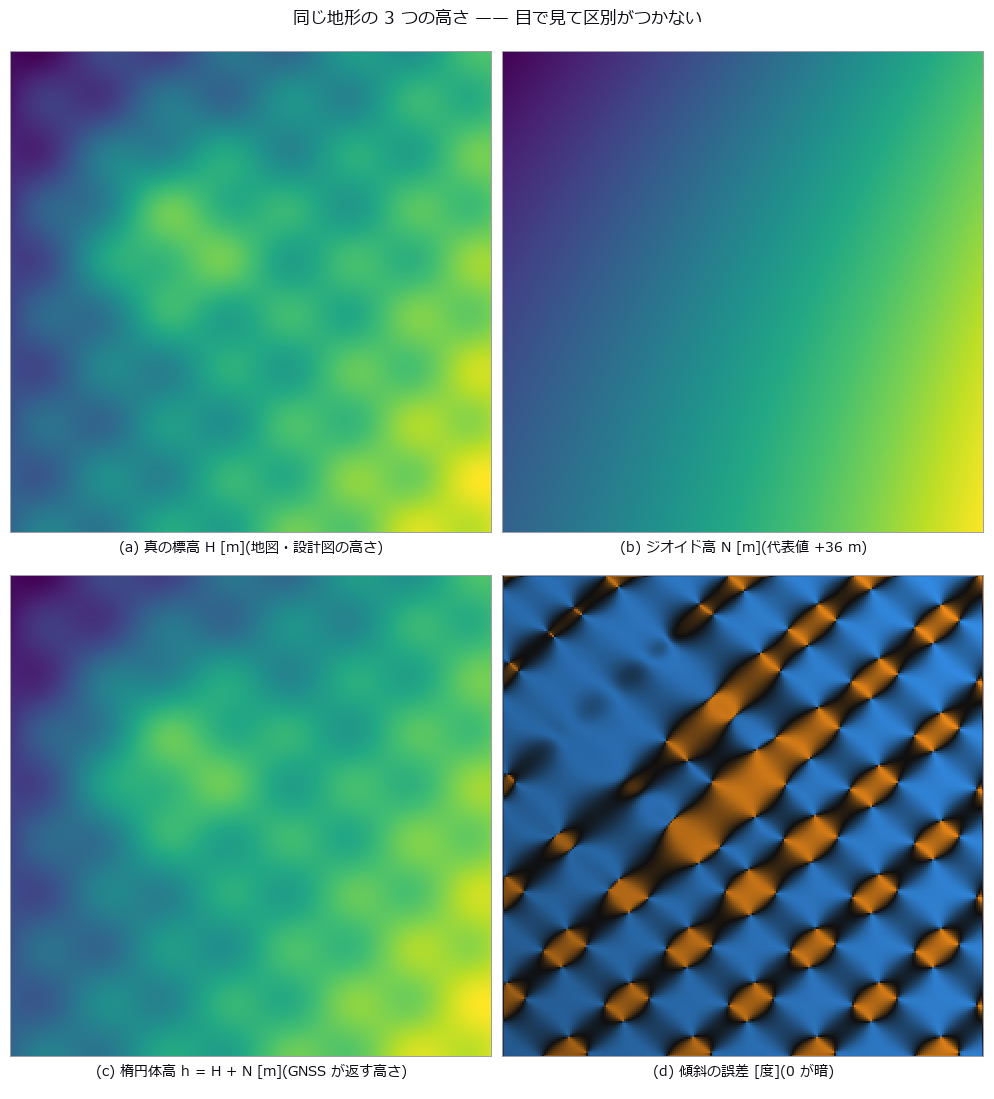
| *↑ Coordinates Go Wrong by Tens of Metres While Still Looking Plausible ―― GNSS returns an ellipsoidal height; maps and drawings use an orthometric one, and the two differ by the geoid undulation — 30 to 40 m around Japan. This exhibit plants a synthetic geoid field and measures which quantities that confusion reaches and which ones it cancels out of. The floor is taken twice: the round trip of the existing operators closes to 1.07e-06 m, and an independent iterative implementation agrees to 7.2e-07 m in latitude — because a round trip alone cannot rule out both directions being wrong the same way. Several closed forms landed: the bound on slope error, atan | grad N | , predicted 0.008771 degrees against 0.008600 measured, with the constant-undulation control at 2.0e-14 degrees, which is exactly zero; the volume error A times the mean undulation agreed to 1.5e-08 cubic metres; the fraction of flat ground whose flow direction reverses was predicted at 76.1 % and measured at 76.2 %. One prediction was badly wrong: the bound on line-of-sight clearance was set at 2.60 m and measured 0.052 m, fifty times smaller, because the linear part of the undulation rides on the sight line and the ground equally and cancels; Earth curvature matters 276 times more. The flat-earth cliff has a closed form but not a single number — at 10 km the prediction of -7.8481 m brackets measurements of -7.8652 m north-south and -7.8303 m east-west, the difference between the meridional and prime-vertical radii. The theme is that the same 36 m is everything or nothing depending on the quantity: it nearly vanishes from differences and survives whole in absolutes, changing an earthwork volume by 3.97e+07 cubic metres and a flooded area from 41.9 % to zero. A control where the design surface is built from the same GNSS shows zero error — a contaminated ruler applied to a contaminated object hides the error. A datum mix-up shifts positions by 446.6 m on average while a relative check between baselines shows only 0.106 m per kilometre, four thousand times less; the danger is not the size but the plausibility. Counting quiet failures against loud ones over a 3600-point global grid, the only mistake that raises is swapping latitude and longitude, and only half the time; radians-for-degrees, a flipped longitude sign, swapped ECEF axes (whose results land in a valid latitude and longitude range 100 % of the time) and feet-for-metres all pass silently. Ten of eleven entries fail quietly. Along the way a real defect was found and fixed: near the Earth’s centre the ECEF-to-geodetic conversion returned a latitude of 180 degrees — a value that does not exist, and one its own inverse rejects.* |
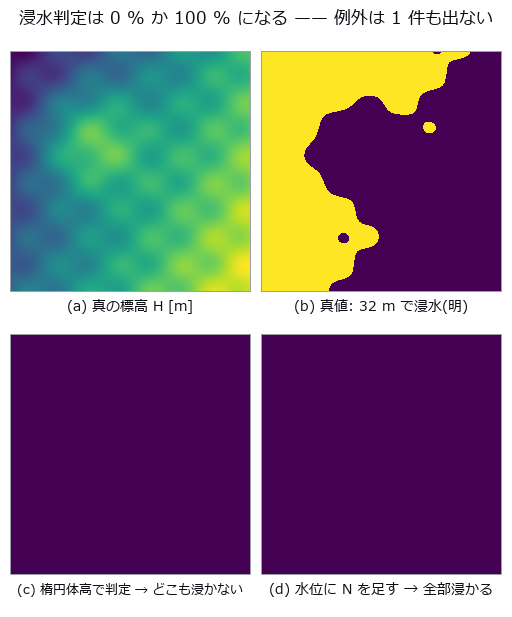
↑ The measurement ―― 分母 58081 セル。真値 24325(41.9 %)に対し、誤用は 0 と 58081。どちらの絵も「もっともらしい」(全面浸水は津波の図に見える)。 (figure labels are in Japanese; the numbers are the same)
py -3.11 examples/poc_geodetic_height_frames.py
Source: examples/poc_geodetic_height_frames.py
Ops used (notes): dem_aspect · dem_earth_curvature_drop · dem_ecef_to_geodetic · dem_flow_direction · dem_geodetic_to_ecef · dem_slope · median
60. Leaf disease severity — colour axes survive the lighting; the grade is decided by the leaf mask and the edge convention
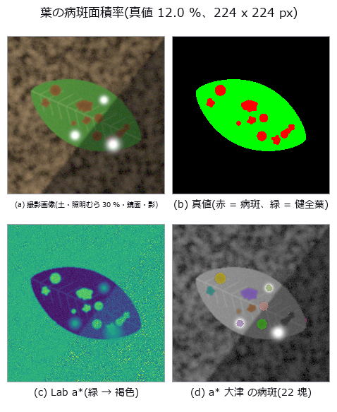
↑ Leaf disease severity — colour axes survive the lighting; the grade is decided by the leaf mask and the edge convention ―― A closed-form leaf outline with lesions of known area, over soil, side lighting, clipped highlights and a shadow, gives ground truth for disease severity (lesion pixels / leaf pixels). A fixed threshold on the green channel (the zero point) is off by +65.2 pt with soil alone; cutting the leaf with the illuminant-projected G and the lesions with Lab a lands at -0.8 pt on the standard scene. Illumination falloff up to 50 % does not move a, but clipped highlights produce only false positives for a (+12.6 pt at 20 % coverage, 0.0 false negatives) versus +2.0 pt for hue, which is invariant to added white. With a 4 px soft lesion edge, choosing the 25 % or 75 % opacity contour as the boundary alone shifts the severity by ±3.5 pt (predicted within 0.4 pt by Steiner’s formula), and of 40 images placed within ±3 pt of a grade boundary, 19-35 are misgraded on soil by every method — on black cloth with a brightness leaf mask, a fixed hue threshold misgrades 8.*

↑ The measurement ―― FN(青)の大きな塊は影と鏡面反射が重なった病斑(葉マスクごと落ちる)。FP(赤)は鏡面反射の下と病斑の縁。 (figure labels are in Japanese; the numbers are the same)
py -3.11 examples/poc_leaf_disease_area.py
Source: examples/poc_leaf_disease_area.py
Ops used (notes): access_channel · blob_features · blob_label · blob_overlay · fill_holes · gaussian · linear_to_srgb · reg_close · reg_erode · rgb_to_lab · select_largest · sk_otsu · specular_free_transform · srgb_to_linear · trans_from_rgb
61. Drone Thermography of a PV Plant — You Think You Are Measuring Temperature Difference, but You Are Measuring Wind and Viewing Angle
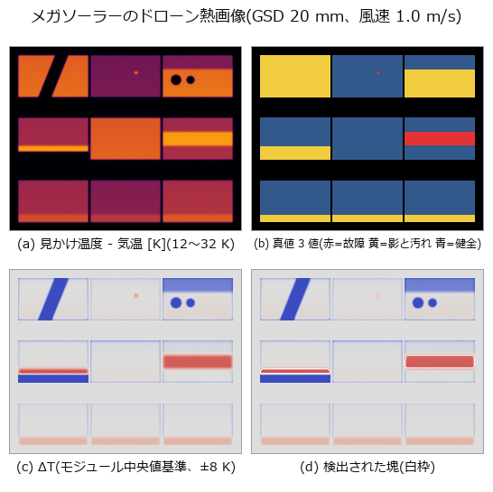
↑ Drone Thermography of a PV Plant — You Think You Are Measuring Temperature Difference, but You Are Measuring Wind and Viewing Angle ―― A megawatt PV array synthesised from a closed-form steady-state heat balance, seeded with known electrical faults (an in-cell hotspot, a bypassed string) and with real-but-not-electrical temperature differences (shading, soiling). A hotspot dissipating 320 W/m² is 11.20 K before dilution yet reaches the camera as 4.23 K — and the dilution comes not from the lateral conduction we expected (x0.960) but from the camera (x0.511). A control scene containing no electrical fault at all still raises 6 blobs when the whole-image mean is the reference (1 healthy, 5 non-fault). The cliff is set by the minimum-area gate rather than the threshold: the hotspot disappears at 1.0 m/s of wind, matching the area-based prediction of 1.1 m/s while the peak-based prediction of 3.0 m/s is wrong. Row-to-row shading warms the sunlit cells of the same string by +4.68 K, only 0.87 K away from the genuine string fault at +5.55 K.

↑ The measurement ―― 「偽」= 故障でも影でも汚れでもない場所に出た塊。しきい値 3.0 K、風速 1.0 m/s。 (figure labels are in Japanese; the numbers are the same)
py -3.11 examples/poc_pv_thermal_survey.py
Source: examples/poc_pv_thermal_survey.py
Ops used (notes): beer_lambert_transmittance · blob_features · blob_label · blob_select · fresnel_dielectric · gauss_filter · median · overlay_mask · surface_form_remove · volume_downsample · warp_by_plane · zoom_image_factor
62. Planting Known Stars in a Real Deep Field — Contamination Lies About the Measurement and the Confidence in the Same Direction
↑ Planting Known Stars in a Real Deep Field — Contamination Lies About the Measurement and the Confidence in the Same Direction ―― Gaussian stars of known flux planted in the real background of the Hubble Deep Field (NASA/STScI, public domain) — the truth is certain because it was planted, and only the background is real. The real sky is not Gaussian: a robust spread of 1,474 e- against a plain standard deviation of 6,698 e- (4.54x), so taking std for noise reports a detection limit 4.5 times too generous. The background is not one number either, ranging 3,176 to 8,448 e- across 195 tiles of 64x64, which leaves up to 3.6 sigma of systematic error after a single global subtraction. Even in the emptiest thirty per cent of the field a fixed amount leaks into the aperture: recovery runs 4.38x at F = 2,000 e- and 1.058x at 100,000, and it is an addition rather than a factor — 1 + C/(F·frac) fits all five points to within 0.9 %, with C = 6,677 e-, a mere 3.0 % of background times effective area. Predicting first that the bias falls below 10 % from 67,521 e- and then measuring there gives 1.086 against the predicted 1.100. In crowded positions the order of magnitude changes, 341x down to 7.80x: a median is robust to outliers, but when half the field is contaminated the median is the contamination. The confidence lies in the same direction — the op reports an SNR of 19.2 where the closed form on the same background gives 4.2 — so gating on S/N passes the contaminated measurements first.
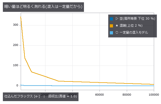
↑ The measurement ―― 開口 1 つあたり C = 6677 e- の足し算として説明できる。 (figure labels are in Japanese; the numbers are the same)
py -3.11 examples/poc_real_sky_photometry.py
Source: examples/poc_real_sky_photometry.py
Ops used (notes): aperture_photometry
63. River surface velocity from an oblique video (LSPIV) — velocity error and discharge error are different numbers
↑ River surface velocity from an oblique video (LSPIV) — velocity error and discharge error are different numbers ―― A power-law surface velocity profile (8 m wide, 1.5 m/s peak) is the ground truth; foam tracers are advected frame by frame and imaged for 60 frames by an oblique bank camera with a known homography, with sky reflection, ripples and noise injected separately. fullseye’s piv_cross_correlate → warp_by_plane (orthorectification) → piv_to_velocity yields u(y) and discharge Q = h∫u dy. The zero point (correlate the oblique frames, convert with one scale) errs +0.31 m/s near bank and -0.28 m/s far bank, the apparent width collapses to 3.3 m and Q is -57 %. Orthorectification gives 0.074 m/s RMS and Q -7.8 %, yet even the control group’s Q -3.0 % is mostly (-2.5 %) the bank trapezoid rule, unrelated to velocity. The tracer-density cliff arrives as outliers, not NaNs (44 % flagged at 0.05 %; ensemble correlation does not rescue the lost windows). Widening the window smears the bank velocity by only -0.008 m/s, orders below the predicted window x gradient, while Q drifts from -1.1 to -7.0 %. Static reflections matter only when fine-grained: the estimate is first pulled (ratio 0.70) then pinned to zero (0.03), and a temporal median restores 0.998. The dt cliff is pair loss, not the quarter rule: removing the search limit leaves the cliff at the same k=4.
↑ The measurement (figure labels are in Japanese; the numbers are the same)
py -3.11 examples/poc_river_surface_velocity.py
Source: examples/poc_river_surface_velocity.py
Ops used (notes): highpass_image · median · piv_cross_correlate · piv_ensemble_correlate · piv_error_stats · piv_outlier_mask · piv_replace_outliers · piv_sample_at_windows · piv_to_velocity · sigma_clip_stack · warp_by_plane
64. Sea-Ice Concentration — The Answer Depends on How Mixed Pixels Are Counted
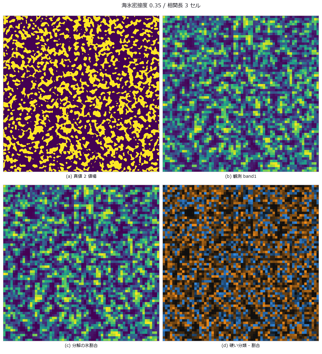
↑ Sea-Ice Concentration — The Answer Depends on How Mixed Pixels Are Counted ―― Ice concentration from a PSF-blurred two-band ice/water image, by hard classification and by linear unmixing. Hard classification is off by -4.2 points, unmixing by +0.02. The bias is explained by the perimeter fraction (R² = 0.984) and crosses zero near a concentration of 0.49 — validate only there and it passes.

↑ The measurement (figure labels are in Japanese; the numbers are the same)
py -3.11 examples/poc_sea_ice_concentration.py
Source: examples/poc_sea_ice_concentration.py
Ops used (notes): blob_features · blob_label · gauss_filter · mat_lstsq
65. Sweep Width — One Number Measured from Aerial Images Decides Whether the Search Works
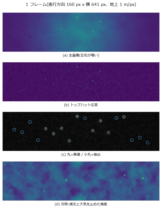
↑ Sweep Width — One Number Measured from Aerial Images Decides Whether the Search Works ―― Measure the lateral range curve p(x) from aerial imagery — detection probability as a function of cross-track distance — and hand its area, W = integral of p dx, to the search plan as the sweep width. This is where image processing and decision-making meet in a single number. The definition itself is demonstrated first: four curves of different shape (the measured p, a rectangle of width W, a triangle of base 2W, and a bimodal curve that cannot see nadir) all scaled to the same area of 256.2 m detect 0.2559 / 0.2563 / 0.2556 / 0.2566 of targets scattered uniformly over a half-width of 500 m, every one within 0.8 sigma of the predicted 0.2562. The shape vanishes; only the area survives. The cliff sits at coverage C = W v t / A = 1, printed in closed form before measuring: min(1, C) = 1.0000 and 1 - exp(-C) = 0.6321, against a rectangular control measuring 1.0000 and 0.6348 (the excess comes from having a finite 64 tracks; the exact value is 0.6350). Four predictions were wrong. Feeding the real p into a parallel sweep gives only 0.8464, not 1.000, because min(1, C) assumes the rectangular definite range law and a curve with tails overlaps its neighbouring tracks. The flatter curve was expected to be the more rectangle-like and therefore stronger, but it was the weaker (0.7705 against 0.8464): rectangle-like means standing inside W without tails, not being flat — while under random search the two curves tie, since random search only sees area. Ground resolution was expected to fall towards the swath edge, but for a nadir-looking central projection it is constant to 0.0e+00 relative spread; what falls is cos^4 vignetting, atmosphere and off-axis blur (an f-theta lens would coarsen the edge by 2.132 times). And subtracting a global background does nothing, because dividing by the whole-frame median and sigma is an affine map that cannot change the ranking (174.4 to 172.0 m); only a per-location subtraction helps (239.6 m). The optimum altitude lands in the interior at 220 m with W = 258.1 +/- 4.0 m, though 220 and 300 m are honestly not resolved apart; with an aircraft whose speed scales as min(1, h/600) the optimum moves to 420 m, so lowering the altitude to raise W does not work. The chaperone here is the false-alarm count, which concentrates at nadir rather than at the edge (113 in the 0-32 m band, zero in the outermost) because targets and whitecaps dim through the same cos^4: the best-seen place barks the most. Moving only the threshold slides W from 406 m to 170 m, so a sweep width quoted without a false-alarm rate says nothing at all.

↑ The measurement ―― 半幅 500 m に一様に撒いた 400000 個。予測 W/2X = 0.2562、モンテカルロの標準偏差 0.0007。 (figure labels are in Japanese; the numbers are the same)
py -3.11 examples/poc_search_sweep_width.py
Source: examples/poc_search_sweep_width.py
Ops used (notes): gauss_filter · gray_tophat · integrate_funct_1d · laplace · ncc_locate · noise_sigma · photon_sample · relative_illumination · star_detect · tophat · vignette · xsk_blob_log
66. Where Is the Edge of a Limb-Darkened Disc? The 50 % Rule Reads the Radius Small
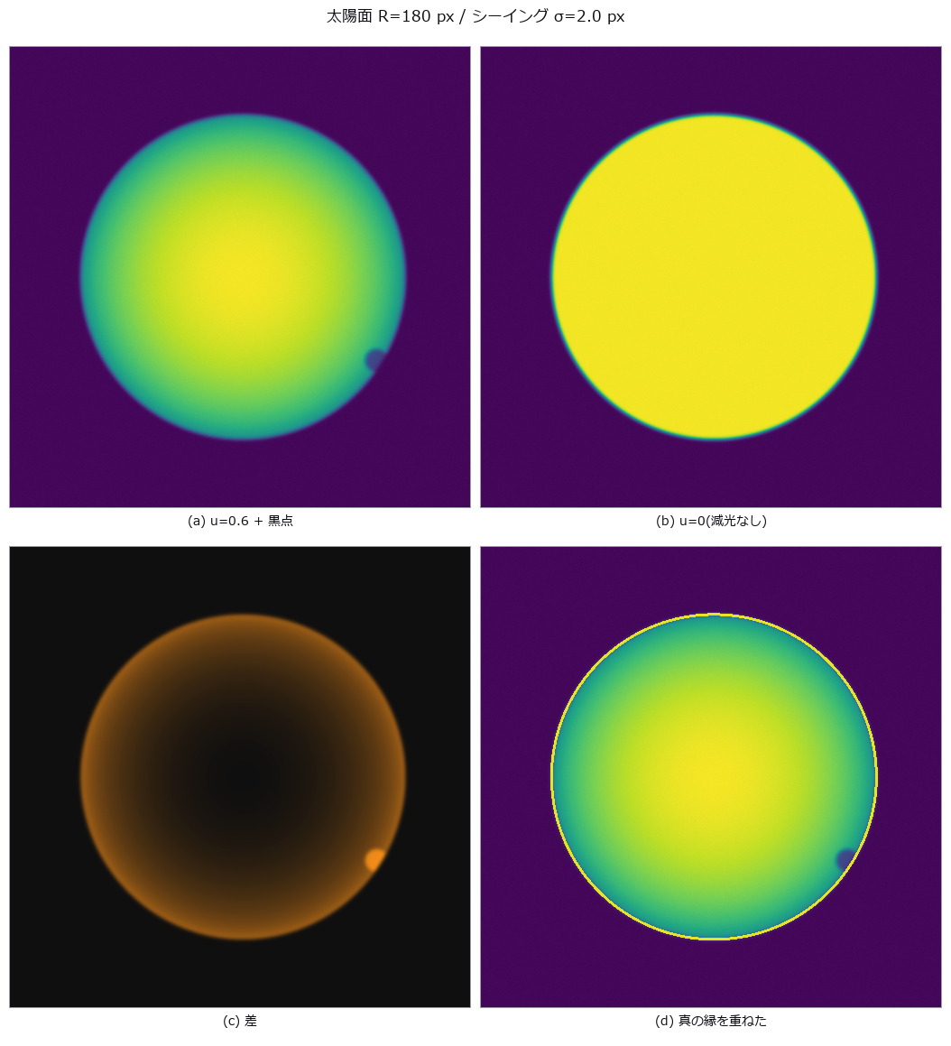
↑ Where Is the Edge of a Limb-Darkened Disc? The 50 % Rule Reads the Radius Small ―― A limb-darkened solar disc seen through seeing, its radius measured by the 50 % rule, by gradient maximum and by model fitting. The prediction ‘bias scales with the darkening coefficient’ failed: at u = 0.8 the bias is -12.76 px (pure geometry predicts -13.14 px). The cancellation point near threshold 0.26, where blur appears to have no effect, moves to 0.38 when u changes.

↑ The measurement (figure labels are in Japanese; the numbers are the same)
py -3.11 examples/poc_solar_limb_darkening.py
Source: examples/poc_solar_limb_darkening.py
Ops used (notes): edge_points · gauss_filter · gaussian · gen_measure_rectangle2 · mat_lstsq · measure_pos
67. To What Fraction of a Pixel Can a Star Be Located, and Where Is the Cliff?
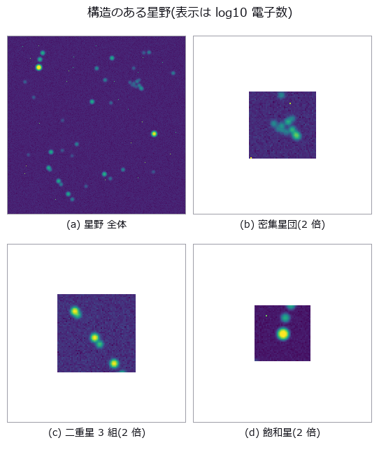
↑ To What Fraction of a Pixel Can a Star Be Located, and Where Is the Cliff? ―― Stars rendered from known celestial coordinates, located by four methods and compared with the Fisher-information bound. At S/N 298 the centroid (null) sits at 5.56x the bound and the background-subtracted centroid at 1.03x; no method beats the bound. At the faint end the null appears to beat it (0.2790 px versus 0.3471 px), but with a sensitivity of 0.038 it is merely returning the rounded initial guess.
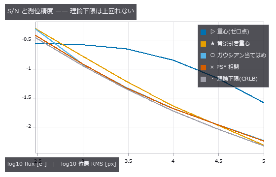
↑ The measurement ―― 暗い端で素の重心が下限を割って見えるのは「動かない推定器」だから(感度 0.038)。 (figure labels are in Japanese; the numbers are the same)
py -3.11 examples/poc_star_astrometry.py
Source: examples/poc_star_astrometry.py
Ops used (notes): gaussian · noise_sigma · psf_fit · star_detect
68. Counting tree rings and extracting the width series — ring count and width correlation fail separately
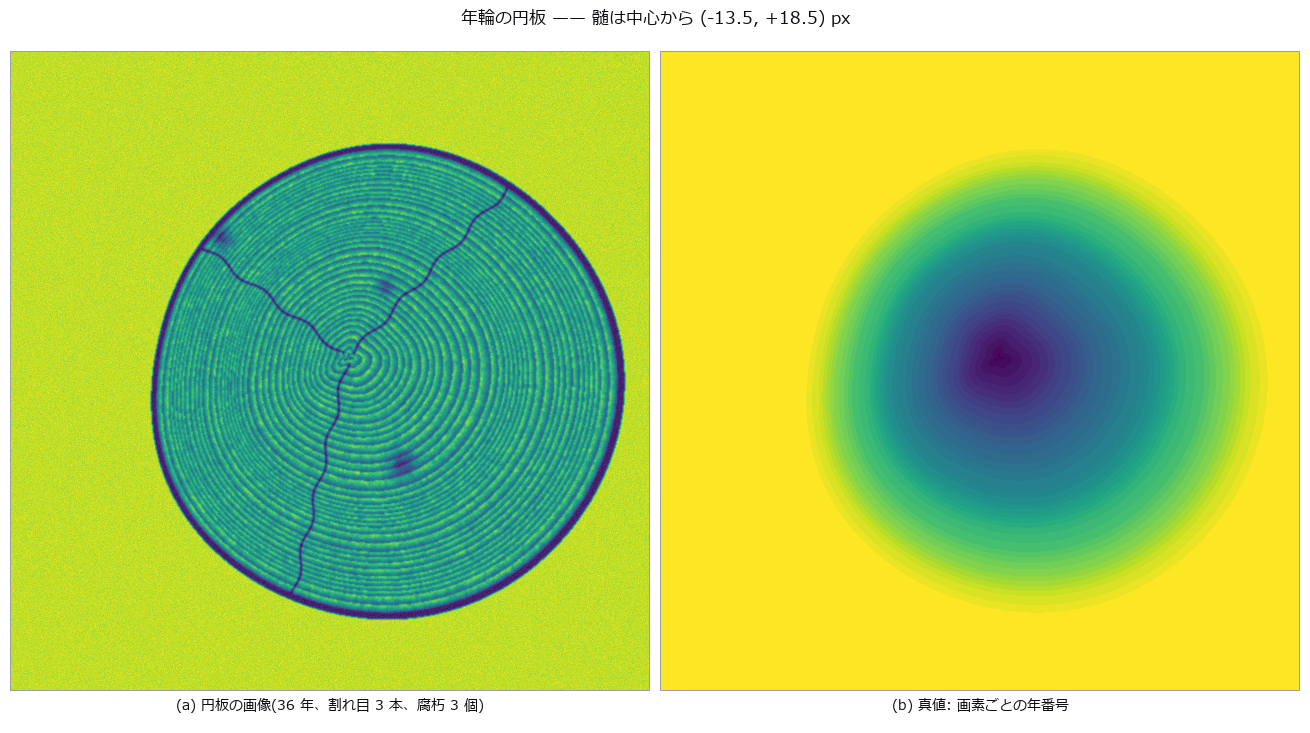
↑ Counting tree rings and extracting the width series — ring count and width correlation fail separately ―― A 36-ring disc is synthesised in closed form with an off-centre pith, eccentric growth, circumferential wobble, wandering cracks, decay spots, grain texture and blur. A single-ray peak count (baseline) gets the ring count right in only 18 of 24 directions, yet the 6 wrong directions still give a width-series correlation of median 0.900. The consensus method (pith-centred polar unwrap, radius normalised by the disc edge, theta-median, 24 sector measure lines, median) returns exactly 36 rings, 0 missing, width correlation 0.996 (mean error 0.13 px). A 20 px pith error leaves the width correlation at 0.994: the cosine modulation lands on the radii (slope -14.9 px), not on the widths (-0.02 px); what it removes is the innermost rings (predicted 2 / measured 2). The thinnest ring is lost at 2.5 px (consensus) and 3.0 px (baseline), and at blur sigma 4 px the baseline counts 13 false rings.

↑ The measurement ―― 偏心成長で境界が θ とともに斜めに走るので、正規化しないとθ 窓の中で外側の年輪がにじむ。 (figure labels are in Japanese; the numbers are the same)
py -3.11 examples/poc_tree_ring_dendro.py
Source: examples/poc_tree_ring_dendro.py
Ops used (notes): derivate_funct_1d · find_peaks · gen_measure_rectangle2 · measure_pos · median_rect · polar_unwrap · smooth_funct_1d_gauss
69. Counting Crop Green — Ground Truth as Per-Pixel Leaf Area Fraction
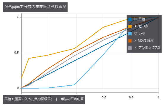
↑ Counting Crop Green — Ground Truth as Per-Pixel Leaf Area Fraction ―― Cover fraction from a four-band field image, scored against the per-pixel leaf area fraction. The null (Otsu on the green channel) overshoots by +16.3 pp at mid-season, and since every method scatters by under 0.5 pp, nearly all of the difference is bias. At emergence on wet soil the null’s cover bias is -0.2 pp while precision and recall are both 0.000 — the number is right and not a single pixel is.
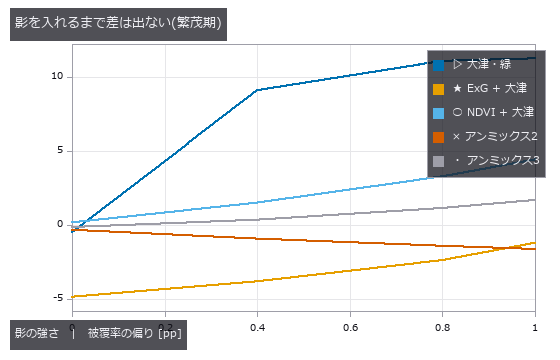
↑ The measurement ―― 影ゼロならゼロ点も悪くない。影は『暗さ』を手掛かりにする手法に直接刺さる。 (figure labels are in Japanese; the numbers are the same)
py -3.11 examples/poc_vegetation_cover.py
Source: examples/poc_vegetation_cover.py
Ops used (notes): cv_otsu · otsu · sk_otsu
70. River Stage From an Oblique Photo — Ignoring Perspective Bends the Row-Number Error Into an Arc
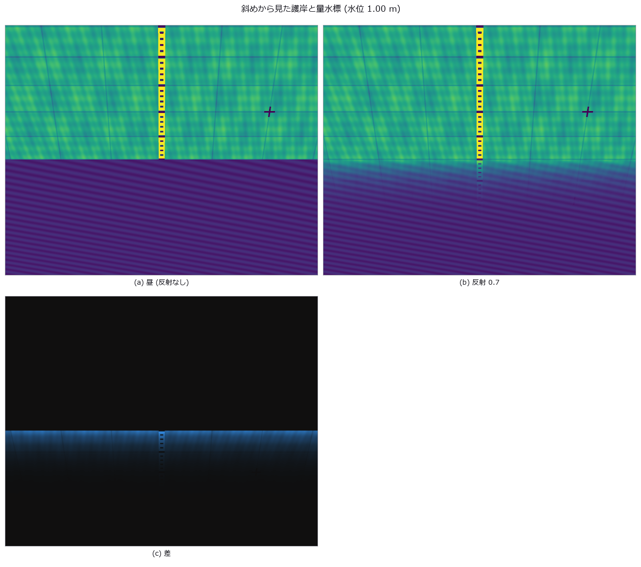
↑ River Stage From an Oblique Photo — Ignoring Perspective Bends the Row-Number Error Into an Arc ―― The waterline detected on an obliquely photographed staff gauge and converted to stage. Linear conversion from two gauge marks bends off by up to -6.4 cm (at 1.00 m), and the sign is decided not by the stage but by whether the reading interpolates (-6.6 cm) or extrapolates (+16.3 cm). A four-point homography brings it under 0.2 cm; what remains is waterline detection, not perspective.
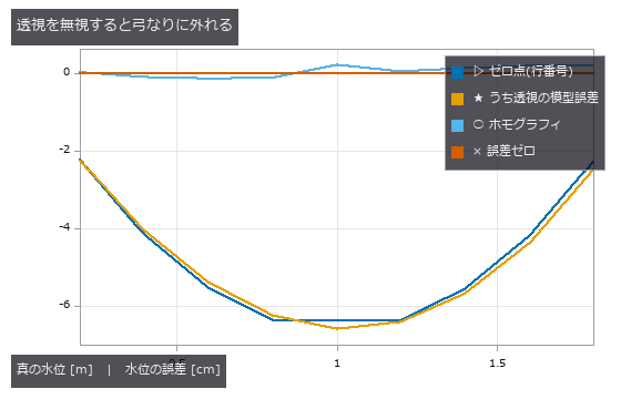
↑ The measurement (figure labels are in Japanese; the numbers are the same)
py -3.11 examples/poc_water_level.py
Source: examples/poc_water_level.py
Ops used (notes): gen_measure_rectangle2 · mat_svd · measure_pos · projective_trans_image · ransac_line · threshold
The Image Quality and Restoration Wing — Looking Better and Getting Closer to the Truth Are Different Things
Deblurring, upscaling, dehazing, focus stacking, reconstructing from projections, ranging by counting photons. Restoration is where ‘it looks better’ and ‘it is closer to the truth’ are most easily confused. The seven exhibits here synthesise the kernel, the depth, the airlight, the PSD, the projections and the arrival time themselves, so the two can be scored separately.
Appearance metrics do not peak at the truth: a hazy input has higher contrast than the true scene; unsharp masking matches the true gradient energy while PSNR drops; adding noise raises PSNR. Conversely, a method can restore stripes finer than Nyquist while PSNR moves by only -0.01 dB.
The null baseline placed throughout is ‘do nothing’. Deblurring with the kernel angle off by 19.4 degrees, FBP from 12 projections, dehazing at visibility above 782 m, depth in textureless regions: each loses to that baseline. Stating the losing conditions in numbers is what this room is for.
71. How Much Camera Shake Can Be Undone — Make the Kernel, Apply It, Invert It, Compare
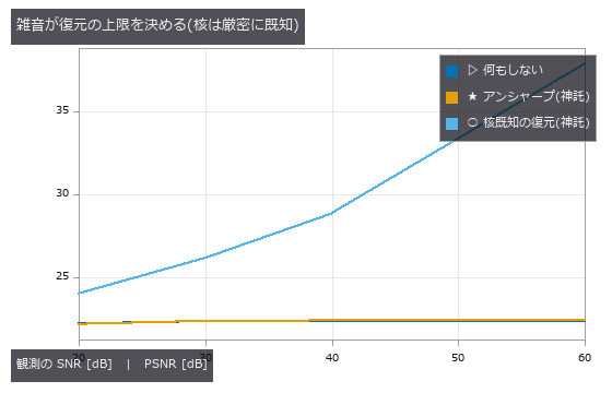
↑ How Much Camera Shake Can Be Undone — Make the Kernel, Apply It, Invert It, Compare ―― A known linear blur kernel applied and inverted, with the ceiling set by noise and by kernel estimation error. Without noise the image recovers from 22.38 to 56.41 dB; at 20 dB SNR the gain is 1.82 dB. A kernel angle off by 19.4 degrees is beaten by doing nothing, and undoing rotational blur with a single kernel makes the centre of rotation worse by -49.41 dB.
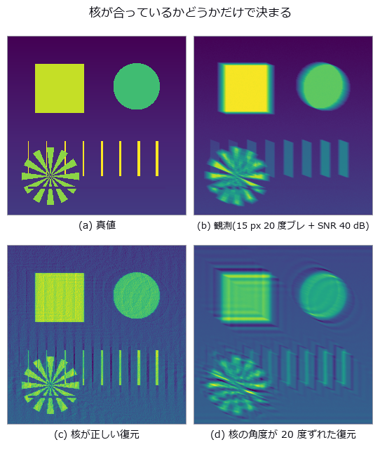
↑ The measurement ―― 4 枚目は「復元した」形をしているが、ゼロ点(観測そのもの)より悪い。絵の見た目では区別できない。 (figure labels are in Japanese; the numbers are the same)
py -3.11 examples/poc_camera_shake_deblur.py
Source: examples/poc_camera_shake_deblur.py
Ops used (notes): psnr · reflect · ssim · unsharp · vol_richardson_lucy
72. Pseudo-colour changes what the reader decides — counting edges that are not there

↑ Pseudo-colour changes what the reader decides — counting edges that are not there ―― A smooth field with provably zero steps was painted and the false edges counted in CIE L and CIEDE2000: jet raises 3, hsv 4, while viridis and gray raise none. Their positions follow in closed form from the sRGB transfer function and the CIE Y weights — jet’s lightness reversals are predicted at 0.3750 / 0.4490 / 0.6250 and measured at 0.3750 / 0.4492 / 0.6250 (max error 0.0002). A real step only out-shouts the false edges above 0.296 %FS with jet versus 0.050 %FS with viridis, matching a prediction made from the colormap LUT alone: jet demands a 5.9x taller step. The value-to-colour mapping matters more than the palette — over a 4.3-decade 1/r^2 field the effective number of distinguishable levels goes from 1.4 (linear) to 76.0 (rank) — and a single outlier costs log 41 % of them (27.4 to 16.3) while percentile and rank are untouched.*

↑ The measurement ―― 平らなら偽の境目は立たない。jet と hsv の山がそのまま『見えてしまう帯』になる。 (figure labels are in Japanese; the numbers are the same)
py -3.11 examples/poc_colormap_readability.py
Source: examples/poc_colormap_readability.py
Ops used (notes): delta_e_map · percentile · rgb_to_lab
73. The Fly’s Compound Eye Is a Light-Field Sensor — Neural Superposition Pays Only Up to the Knee
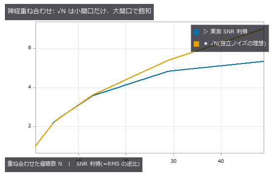
↑ The Fly’s Compound Eye Is a Light-Field Sensor — Neural Superposition Pays Only Up to the Knee ―― A 9×9 plenoptic synthesis of the ommatidial array, measuring the SNR gain when the same point is pooled over N ommatidia. For small apertures √N holds almost exactly (N=5: 2.25 vs 2.24), but for large ones the interpolation error does not average out and the gain saturates (N=49: 5.33 vs 7.00). The fly’s six-fold pooling of R1–R6 sits below the knee. Depth comes from the array (near +1.998, far +0.499 against true 2.00 / 0.50), and a minority occluder is seen through by median pooling (RMS on hidden pixels: single view 0.237 → mean 0.065 → median 0.025).
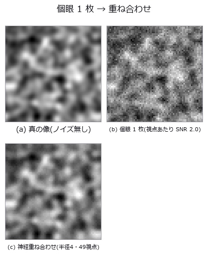
↑ The measurement (figure labels are in Japanese; the numbers are the same)
py -3.11 examples/poc_compound_eye.py
Source: examples/poc_compound_eye.py
Ops used (notes): lf_all_in_focus · lf_aperture_mask · lf_depth_from_focus · lf_plenoptic_design · lf_subaperture · lf_synthesize · lf_synthetic_aperture · median
74. Where CT Reconstruction Starts to Break as Projections Are Removed
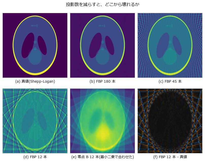
↑ Where CT Reconstruction Starts to Break as Projections Are Removed ―― Shepp-Logan re-imaged with 180 down to 12 projections, FBP placed beside two nulls: a blank image and unfiltered back-projection. With 12 projections FBP (RMSE 0.2576) is worse than the blank image (0.2420). A check that never looks at the reconstruction — the row sums of the sinogram — caught a -3.34 % mass loss that RMSE could not see; fixing the ramp filter’s DC bin brought it to -0.0099 %.
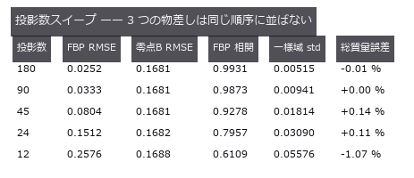
↑ The measurement ―― RMSE で見ると 12 本は空白画像 0.2420 より悪い。相関とストリークは別のことを言う。 (figure labels are in Japanese; the numbers are the same)
py -3.11 examples/poc_ct_fidelity.py
Source: examples/poc_ct_fidelity.py
Ops used (notes): backproject_sinogram · ellipse_phantom · ellipse_sinogram · filtered_backprojection · projection_angles · radon_transform · rmse · ssim · stat_correlation
75. Removing Haze — Ground Truth From the Scattering Model, Transmission and Airlight Scored Apart
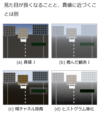
↑ Removing Haze — Ground Truth From the Scattering Model, Transmission and Airlight Scored Apart ―― A hazy image built from depth, airlight and extinction so that the true transmission and the true scene are both known, then dehazed and scored. The overall +4.04 dB hides a -1.49 dB degradation of the near field covered by +4.03 dB mid and +11.28 dB far. Above 782 m visibility dehazing does harm, and adding noise raises PSNR (an accidental cancellation).
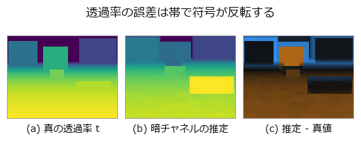
↑ The measurement ―― 空では過大評価(明るい側)、近景では過小評価(暗い側)。全体の平均バイアスでは打ち消し合って見えない。 (figure labels are in Japanese; the numbers are the same)
py -3.11 examples/poc_dehazing.py
Source: examples/poc_dehazing.py
Ops used (notes): clahe · equalize · image_entropy · joint_bilateral · psnr · rank_image · ssim
76. Ranging by Counting Photons — How Many for How Many Millimetres?
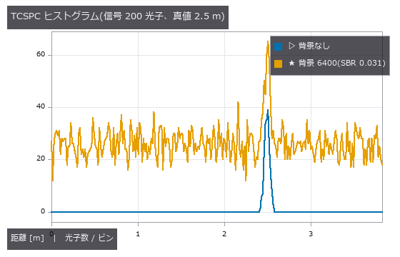
↑ Ranging by Counting Photons — How Many for How Many Millimetres? ―― Range read from an arrival-time histogram built by bin-integrating a Gaussian at the round-trip time and drawing Poisson samples. With 200 photons the raw peak position errs by 11.02 mm and the gated centroid by 2.29 mm, riding the 31.83 mm/√N bound at 1.00 to 1.07x. With background the plain centroid collapses by two orders (564 mm at SBR 0.031), and the family’s recommended Gaussian fit at 8.82 mm loses to a gated centroid a user can write in six lines.
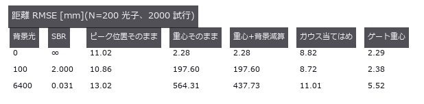
↑ The measurement ―― 背景が無ければ素の重心で足りる。背景が入ると 2 桁崩れ、docstring が勧める背景減算でも戻らない。 (figure labels are in Japanese; the numbers are the same)
py -3.11 examples/poc_dtof_ranging.py
Source: examples/poc_dtof_ranging.py
Ops used (notes): dtof_cube_depth · dtof_cube_simulate · dtof_depth · gaussian · median · tcspc_background_subtract · tcspc_coates_correct · tcspc_simulate
77. The Fly’s Visual Front End as a Chain of Operators — Turning and Walking Through a Synthetic Sky, What Can and Cannot Be Read
| *↑ The Fly’s Visual Front End as a Chain of Operators — Turning and Walking Through a Synthetic Sky, What Can and Cannot Be Read ―― One eye assembled from a 721-ommatidium hexagonal lattice → acceptance function → lamina DC removal → Hassenstein-Reichardt correlators → HS opponent sum, turning under a 1/f banded sky. The direction and waveform of self-rotation are readable (correlation with the true yaw rate +0.785, +0.880 with a membrane low-pass, sign agreement 0.92), but skipping the lamina DC removal makes the correlator emit a DC × high-pass ripple and the correlation drops to +0.504. Walking forward without turning, the full-field readout turns into a −0.689 ‘rotation’; restricting to the upper field still leaks −0.221 because acceptance functions straddle the horizon (0.000 above el = 2Δρ). The opponent ratio discards speed, so a 1.4°/s flow from a dome 20 m away reads −0.612. The LGMD η peak comes α·l/ | v | before collision (−0.1570 s, predicted −0.1567 s) at θ = 23.97° (predicted 24.02°; 24.6° for the exact subtense of a sphere, a quartic root), the sphere τ rides d/ | v | with RMS 1e-5 s, and the disk formula misapplied to a sphere reads cos²(θ/2) = 0.75× at 60°. Twelve grating directions give DSI 0.798 with preferred direction 0°.* |
↑ The measurement ―― 相関 +0.785(膜 LP つき +0.880、ラミナ段なし +0.504)。対向比は符号の一致度なので、尺度 k は最小二乗で合わせてある。 (figure labels are in Japanese; the numbers are the same)
py -3.11 examples/poc_fly_vision.py
Source: examples/poc_fly_vision.py
Ops used (notes): fly_dsi · fly_emd_response · fly_hex_lattice · fly_hex_resample · fly_hs_readout · fly_lgmd_eta · fly_sky_1f · fly_tau_from_expansion
78. Focus Stacking — The All-in-Focus Image and the Depth Map Are Different Things
↑ Focus Stacking — The All-in-Focus Image and the Depth Map Are Different Things ―― An all-in-focus image and a depth map pulled from 15 frames blurred by the closed-form circle of confusion. The all-in-focus image reaches 35.89 dB (null 20.98 dB), yet the depth from the same fusion loses to the null by 8x (0.13x) in textureless regions. A relative confidence scores 0.9923 there, higher than the 0.9630 of textured regions; rejecting by absolute value (23600x apart) brings the RMS from 1.505 to 0.878 mm.
↑ The measurement ―― 左下の無テクスチャの四角だけ、誤差が掃引全域にばらけた乱数になっている(段差帯のハローも見える)。 (figure labels are in Japanese; the numbers are the same)
py -3.11 examples/poc_focus_stacking.py
Source: examples/poc_focus_stacking.py
Ops used (notes): csi_height_map · defocus_blur · dilation_circle · fuse · gauss_filter · laplace · mean_image · optical_camera · psnr · sobel_amp · xcv2_lap_var
79. Depth From a Light Field — A Light Field of Known Depth, Confronted With Its Nulls
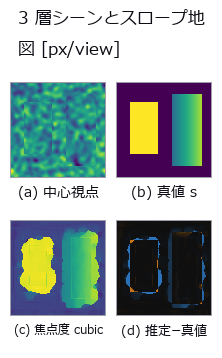
↑ Depth From a Light Field — A Light Field of Known Depth, Confronted With Its Nulls ―― A 9×9 light field rendered by analytic inverse mapping, with focus-measure, EPI-slope and two-view block matching scored against the true slope map. The winner beats the constant null by 22x, but beats two-view matching — which uses only 2 of the 81 views — by just 1.6x, and only with cubic interpolation. The default linear interpolation snaps to integer slopes, reading a true 1.30 as 1.4750 (11.9 % in depth).
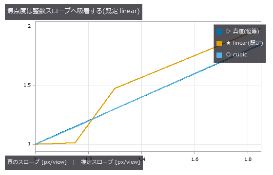
↑ The measurement ―― linear は 1.08/1.15 を 1.0 へ、1.85 を 2.0 側へ引く。cubic は恒等線に乗る。生成側の補間はゼロ(Fourier シフト)。 (figure labels are in Japanese; the numbers are the same)
py -3.11 examples/poc_lightfield_depth.py
Source: examples/poc_lightfield_depth.py
Ops used (notes): lf_depth_from_focus · lf_disparity_to_depth · lf_epi · lf_epi_slope · lf_refocus
80. Deblurring a Real Photograph — Three Rulers, Three Different Winners
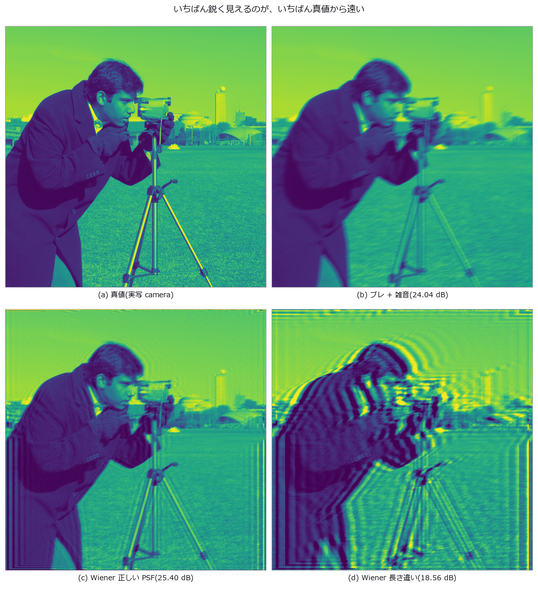
↑ Deblurring a Real Photograph — Three Rulers, Three Different Winners ―― The truth here is a real photograph (scikit-image camera, CC0) and only the degradation is planted: a straight 11-pixel blur at 20 degrees plus noise of sigma 0.004. Doing nothing scores 24.04 dB, and a Wiener filter at the commonly used nsr of 0.005 scores 23.66 — it loses to the null. Stopping there would be misrepresenting the method: sweeping nsr gives 19.18 dB at 0.0005 and 25.40 dB at 0.02, so a fixed knob is not a comparison at all. The knob moves the result by 6.22 dB while deconvolving at all is worth 1.36 dB, a factor of 4.6 — the setting matters more than the method. Applying three rulers to the same seven results puts three different methods first: PSNR picks the correct-PSF Wiener at 25.40 dB, gradient energy picks motion_deblur at 0.2986, which is 1.54 times the truth’s own 0.1936 — an image sharper than the truth wins — and blur_effect picks unsharp. The methods those reference-free rulers choose cost 4.98 dB and 3.26 dB against the best. In fairness, blur_effect does rank the truth itself above every method: it measures blur correctly and still loses you three decibels when used to choose. Mistaking the blur length as 21 instead of 11 costs 5.48 dB against doing nothing while raising the gradient energy to 1.37 times the truth, so it looks like it worked. The cliffs: at sigma 0.016 the gain falls to 0.05 dB, and the gain over blur length peaks at 5 pixels, falling at both ends because a short blur has little to remove and a long one has destroyed the information.
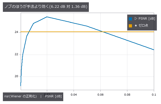
↑ The measurement ―― 固定した nsr で比べると、正しい PSF でもゼロ点に負ける。 (figure labels are in Japanese; the numbers are the same)
py -3.11 examples/poc_real_deblur_honesty.py
Source: examples/poc_real_deblur_honesty.py
Ops used (notes): iv_motion_deblur · iv_richardson_lucy · iv_unsharp_deblur · psnr · reflect · sk_blur_effect · unsharp
81. Does Super-Resolution Add Information? Downsample With the Truth in Hand, Restore, Count
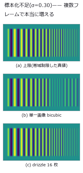
↑ Does Super-Resolution Add Information? Downsample With the Truth in Hand, Restore, Count ―― Observations made by downsampling the truth, with single-image upscaling, iterative back-projection and drizzle scored on a resolution table. No single-image upscaler beats the bicubic null by more than +0.036 dB. Drizzling 16 sub-pixel-shifted frames gains +13.96 dB in the undersampled condition, and the modulation of a period-6 pattern beyond Nyquist rises from 0.03 to 0.38.
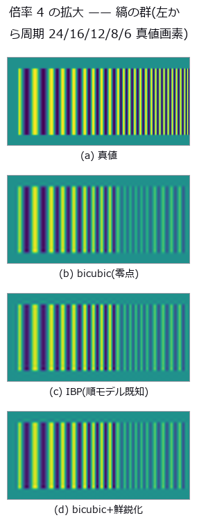
↑ The measurement ―― 鮮鋭化だけがナイキスト(周期 8)より細かい列にも縞を作る。それは分解能ではなく無い縞。 (figure labels are in Japanese; the numbers are the same)
py -3.11 examples/poc_superresolution_limits.py
Source: examples/poc_superresolution_limits.py
Ops used (notes): drizzle_resample · piv_cross_correlate · psnr · ssim · unsharp · vol_fft_lowpass · vol_resize · volume_downsample
The Time-as-3-D Wing — A Video Is One Volume
Treat a 2-D video as one (t, y, x) volume and the 3-D ops — connected components, isosurfaces, region properties — work along time unchanged. Merging colonies become a Y in space-time, passing vehicles become bands in a (t, x) image, a wavefront’s arrival time becomes an isosurface. The six exhibits here demonstrate exactly that.
The time axis also brings its own traps. Rounding onto the frame grid always delays; pixel area makes merging look early. Mislinks come in two opposite kinds, so a single error rate cannot say which way the diffusion coefficient is wrong. Template tracking drifts quietly before it ever loses the target, and all 152 drifted frames report ‘found’.
The motion-magnification exhibit carries the most candid conclusion in the room: exact to machine precision up to a magnification of 200, and of no help for measurement. Magnification is a tool for showing people, not for measuring.
82. Modal identification from video — frequency survives to the end, damping lies first
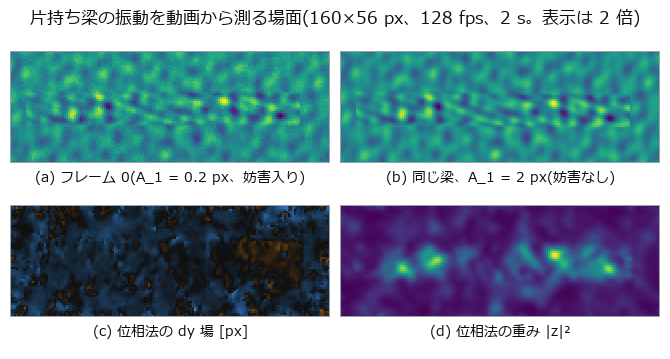
↑ Modal identification from video — frequency survives to the end, damping lies first ―― A cantilever beam (closed-form Euler–Bernoulli modes) decaying freely in three modes is rendered into video with sensor noise, 100 Hz lighting flicker, camera shake and rolling shutter, then identified with phase-based displacement (phase_displacement) and PIV (piv_cross_correlate). All three natural frequencies come out within 0.06 Hz, but the damping ratio of mode 1 from the very same series is 0.0778 (half-power), 0.0188 (envelope) or 0.0181 (fit) against a true 0.02. Sweeping the amplitude from 0.02 to 2 px, the quantities break in the order f → ζ → MAC_2 → MAC_3: at 0.02 px the phase method still has f_1 within +0.030 Hz while ζ_1 is 0.23 of the truth. At 48.5 fps the flicker alias lands exactly on f_1 = 3.00 Hz; a single-pixel brightness zero-point cannot report ζ at all, while the phase method survives at 0.0191.
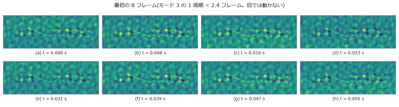
↑ The measurement (figure labels are in Japanese; the numbers are the same)
py -3.11 examples/poc_beam_modal_video.py
Source: examples/poc_beam_modal_video.py
Ops used (notes): envelope · phase_displacement · piv_cross_correlate · temporal_bandpass
83. The Cold-Chain Temperature Record — Where You Taped the Logger Is the Verdict
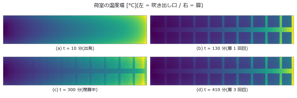
↑ The Cold-Chain Temperature Record — Where You Taped the Logger Is the Verdict ―― Twelve hours of a 12.0 m x 2.4 m reefer hold, built as a single (t, y, x) volume of 720 min x 60 x 12 cells with known closed-form physics: distance from the supply vent, infiltration from each of the four walls, five door-opening pulses, and first-order thermal lag (5 min for air, 64-91 min for product). 108 of 490 product cells (22.0 %) truly fail, yet a single logger taped in the product reports PASS for 82.4 % of the placements. Turning the causes off one at a time separates the failure modes: walls alone give 95.5 % false passes and 0.0 % false alarms, while walls off and doors on drop true failures to 2.0 % but raise false alarms to 3.5 % — and a logger in the product then passes 100 % of the time, because short pulses never enter the product. The cliffs can be predicted on paper: the time-constant cliff measured at 19-138 min matches a two-stage (hold air + logger) model within 18 % relative, and the sampling-interval and 0.5 K quantisation cliffs match their predictions exactly. Converted to “minutes allowed at 12 °C”, the three metrics computed from the same record differ by 4.6x (60 / 276 / 197 min) and disagree on the verdict at 82 of 720 placements (11.4 %).
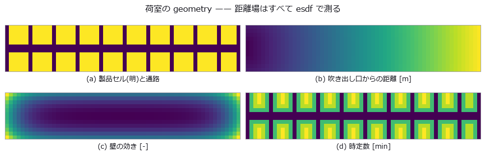
↑ The measurement (figure labels are in Japanese; the numbers are the same)
py -3.11 examples/poc_cold_chain_excursion.py
Source: examples/poc_cold_chain_excursion.py
Ops used (notes): esdf · integrate_funct_1d · render_volume_projection · sample_funct_1d · vol_label · vol_label_shape_stats · vol_mip · vol_profile_line · vol_region_props
84. Measuring the Growth, Not the Width — Rephotographing the Same Wall Changes What the Error Is
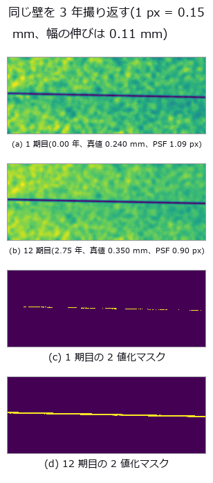
↑ Measuring the Growth, Not the Width — Rephotographing the Same Wall Changes What the Error Is ―― A wall at 1 px = 0.15 mm, rephotographed for twelve epochs over three years, with a crack opening at a true 0.040 mm/yr. Thresholding and counting pixels understates the width by 25.0 % yet overstates the growth rate by +153.0 %, and invents +0.0117 mm/yr of growth in a control where the width is frozen (the culprit is blur, isolated by switching one nuisance at a time). Integrating the intensity deficit gives +3.1 % on the rate and +0.0005 mm/yr on the control. The thresholded rate swings from 0.0241 to 0.1038 mm/yr on initial width alone — it depends on whether a one-pixel step happens to fall inside the observation window.
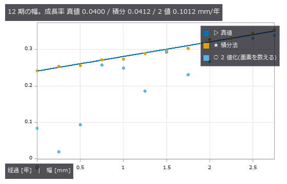
↑ The measurement ―― 2 値化は幅の偏りより期ごとの跳ねが問題。跳ねの正体はぼけと画素位相で、4 節と 3 節で分けて数える。 (figure labels are in Japanese; the numbers are the same)
py -3.11 examples/poc_crack_width_timeseries.py
Source: examples/poc_crack_width_timeseries.py
85. Micro-Vibration of a Structure From Video — Does Motion Magnification Help You Measure?
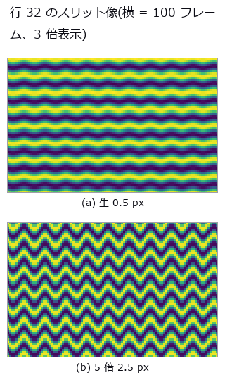
↑ Micro-Vibration of a Structure From Video — Does Motion Magnification Help You Measure? ―― A vibration of known amplitude 0.02 px at 3.7 Hz, synthesised to test whether motion magnification helps measurement. Exact to machine precision up to α = 200. But magnification does not improve measurement precision — multiplying the phase by α multiplies the noise by α. On a cantilever, phase correlation returns 0.15 px, the area average of 0.30 and 0.00 px, a number that exists nowhere.
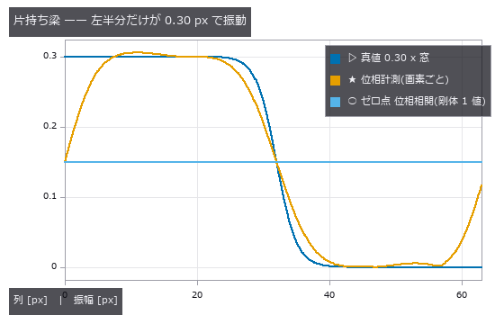
↑ The measurement ―― 剛体を仮定する位相相関が返す 0.150 px は 0.30 と 0.00 の面積平均で、どの列の真値とも違う。 (figure labels are in Japanese; the numbers are the same)
py -3.11 examples/poc_motion_magnification.py
Source: examples/poc_motion_magnification.py
Ops used (notes): band_snr · displacement_series · motion_magnify · phase_displacement · synthesize_translation · temporal_band_power · temporal_bandpass
86. Particle Tracking as a (row, column, time) Volume — Mislinks Come in Two Directions
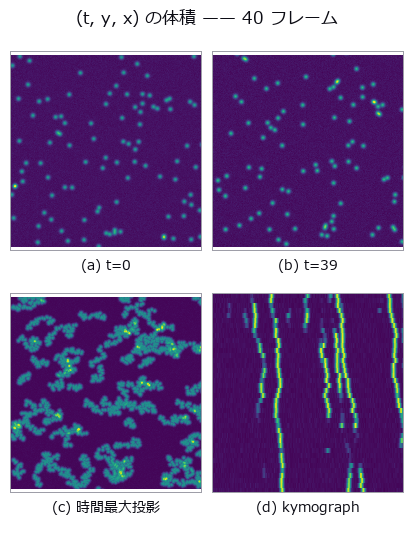
↑ Particle Tracking as a (row, column, time) Volume — Mislinks Come in Two Directions ―― A video of 400 particles tracked, with the diffusion coefficient D read from the trajectories. Ambiguous mislinks pull D down to 0.925x; mislinks caused by missing targets push it up to 3.429x in the same video — one error rate cannot tell you the direction. What helps is not a one-to-one constraint but a single line imposing a maximum link distance (3.429 → 1.304).
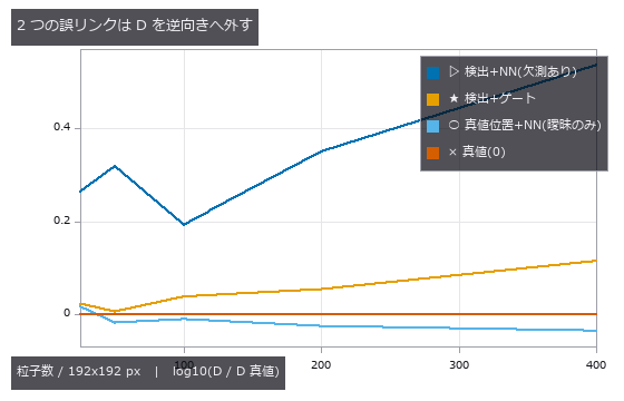
↑ The measurement ―― 縦軸は常用対数(0 が真値)。欠測は遠い他人を掴んで D を上げ、曖昧は近い相手を選んで D を下げる。上限距離のゲート 1 行で上向きの暴走が 1/2.6 に。 (figure labels are in Japanese; the numbers are the same)
py -3.11 examples/poc_particle_tracking.py
Source: examples/poc_particle_tracking.py
Ops used (notes): blob_features · blob_label · vol_label · vol_local_maxima
87. Did It Settle, or Did We Just Scan It Again — What Changes When You Cut at the Detection Limit
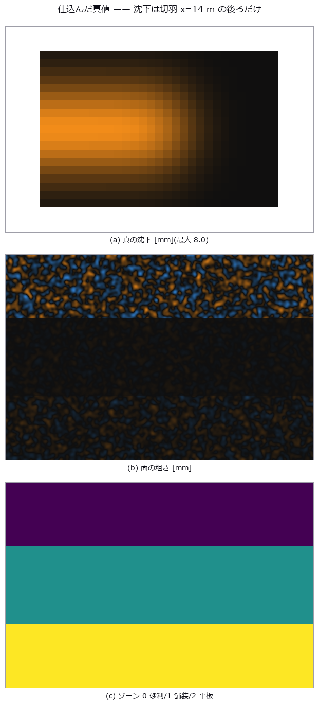
↑ Did It Settle, or Did We Just Scan It Again — What Changes When You Cut at the Detection Limit ―― A 24 x 16 m road surface settling above a tunnel drive, measured from two epochs of point cloud. The nearest-neighbour baseline (C2C) returns a median of 47.74 mm even with zero change — that is just the point spacing — and carries no sign. M3C2 averages -2.43 mm, matching the truth, but only 275 of 551 cores (49.9 %) exceed their level of detection, and those average -4.34 mm: the single averaged number agrees with neither. LoD is a map of the surface, not of the settlement, ranging 0.51 to 3.58 mm across zones. Summing only the significant cores shrinks the volume from 0.8569 to 0.7643 m3, and that shortfall is predictable in advance from the per-core LoD (0.867 predicted versus 0.892 measured).
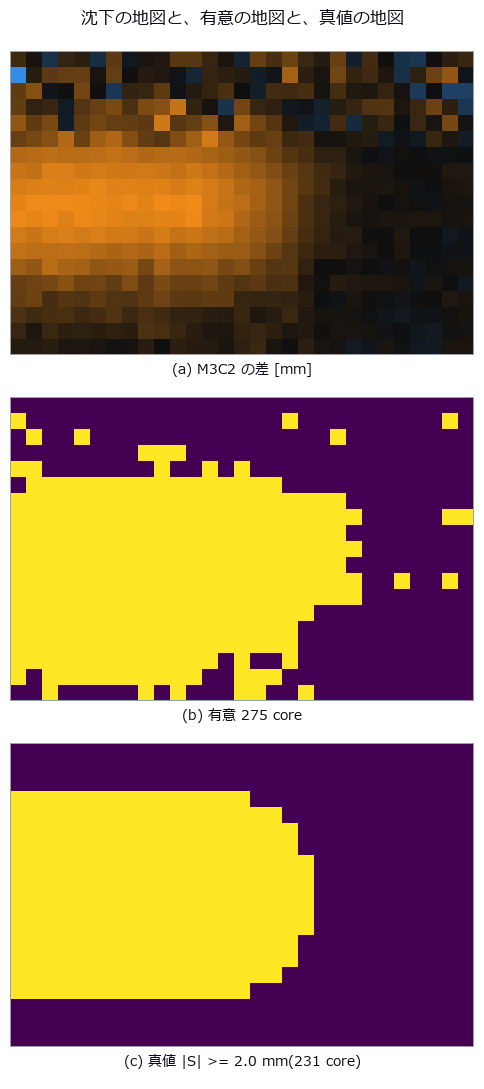
↑ The measurement ―― 有意の地図は真値の地図をよく復元する(TPR 88.7 % / FPR 3.6 %)。ただし縁が痩せる —— そこが 7 節の体積の話。 (figure labels are in Japanese; the numbers are the same)
py -3.11 examples/poc_settlement_significance.py
Source: examples/poc_settlement_significance.py
88. Template Tracking Drifts Quietly Before It Ever Loses the Target
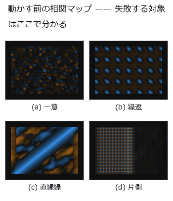
↑ Template Tracking Drifts Quietly Before It Ever Loses the Target ―― A camera moved by a known similarity transform, exposing the three ways template tracking fails: losing the target, drifting quietly, and being confidently wrong. All 152 of the 152 drifted frames passed the peak threshold calibrated without occlusion and reported ‘found’. The only absolute quantity measurable without ground truth is forward-backward inconsistency.
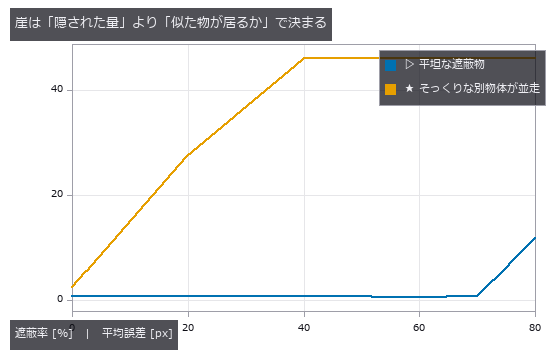
↑ The measurement ―― 同じ遮蔽率でも、そっくりな別物体が視野に居るだけで崖がはるかに手前へ来る。 (figure labels are in Japanese; the numbers are the same)
py -3.11 examples/poc_template_tracking.py
Source: examples/poc_template_tracking.py
Ops used (notes): ncc_locate · reflect · shape_locate
89. A Growth Time-Lapse as Space-Time Connected Components
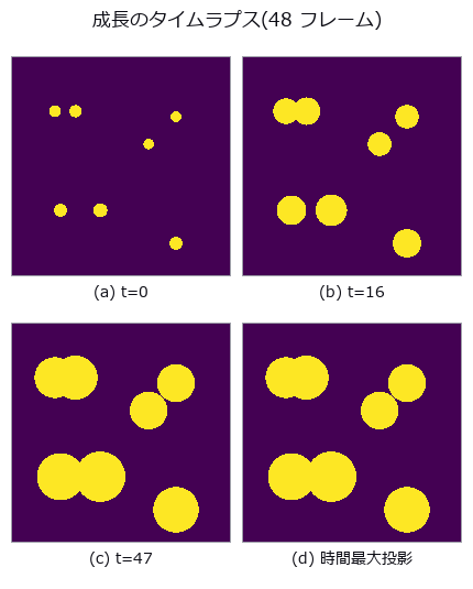
↑ A Growth Time-Lapse as Space-Time Connected Components ―― A video of colonies spreading and merging, read as a (t, y, x) volume with 3-D connected components. Pixel area makes merging look early (-1.16 frames for pair 0-1) while rounding onto the frame grid makes it look late (+0.94); the two oppose, so the sum looks small. The default 26-connectivity of vol_label merged a near miss with a gap of 0.92.
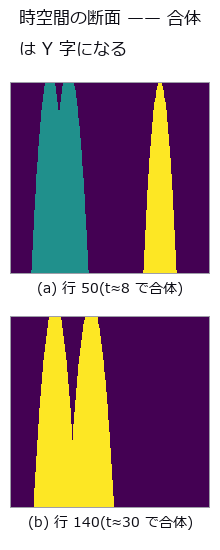
↑ The measurement ―― 縦が時間(下向き、4 倍に拡大)、横が列。2 本の管が合わさる高さがそのまま合体時刻。色は 3-D ラベル。 (figure labels are in Japanese; the numbers are the same)
py -3.11 examples/poc_timelapse_growth.py
Source: examples/poc_timelapse_growth.py
Ops used (notes): blob_label · vol_label · vol_region_props
90. Counting in (x, y, t) — Vehicles Passed, Occlusion, and One Constant: L/V
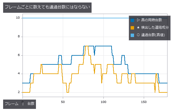
↑ Counting in (x, y, t) — Vehicles Passed, Occlusion, and One Constant: L/V ―― A synthetic traffic video counted per frame, by a virtual loop, and by connected components in a (t, x) slit image. The per-frame maximum reports 7 for 10 vehicles passed — it measures a different quantity. All three failure conditions are written with one constant, vehicle length over speed = L/V (9.0 frames); at a frame interval of 16 the bands fragment and 10 vehicles become 49.
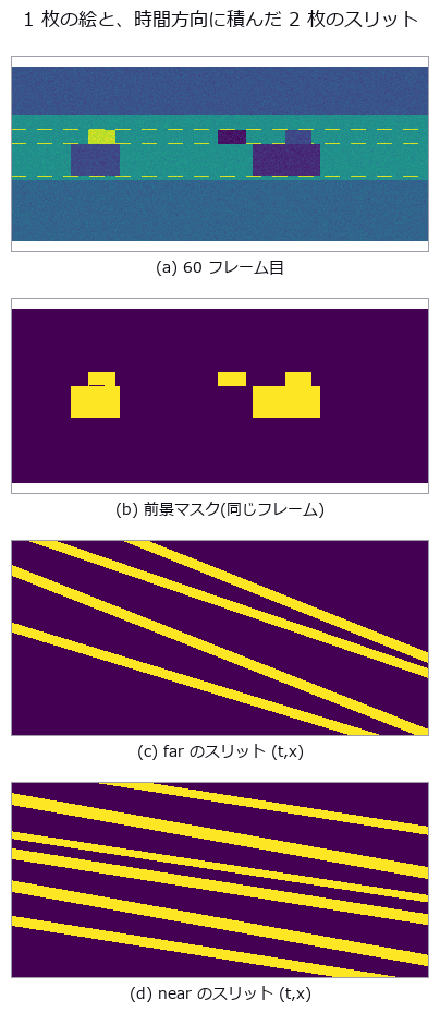
↑ The measurement (figure labels are in Japanese; the numbers are the same)
py -3.11 examples/poc_traffic_counting.py
Source: examples/poc_traffic_counting.py
Ops used (notes): blob_features · blob_label · threshold
91. Where the Warehouse Dwell Came From — Count Waiting Without Its Kind and Everything Is Just Congestion
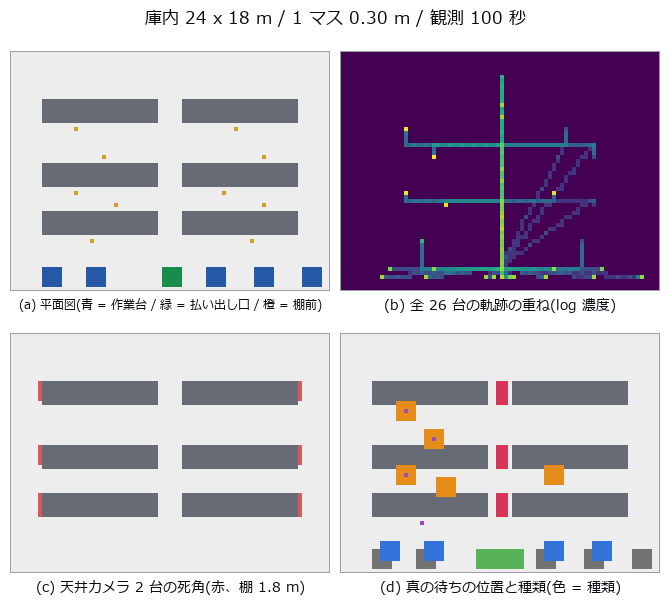
↑ Where the Warehouse Dwell Came From — Count Waiting Without Its Kind and Everything Is Just Congestion ―― A synthetic warehouse floor plan with 26 tracked workers and AGVs, in which replenishment waits, queueing, aisle interference, system waits and stockouts were planted with known times and durations, then read as one (t, y, x) volume. Of the naive 321.5 s of “total dwell”, only 198.0 s (61.6 %) is real waiting; the rest is productive work and creep. Removing all queueing or all aisle interference moves that single number by -39.0 s versus -38.0 s, so it cannot say which to fix, while the per-kind counts drop to zero only for the kind that was removed. A stockout moves dwell by -17.0 s but adds 94.6 m of walking, and the three degradation axes each kill a different kind: sampling interval kills the short waits, occlusion kills the waits pressed against racks, and ID merging kills the two kinds defined by a relation between two people.
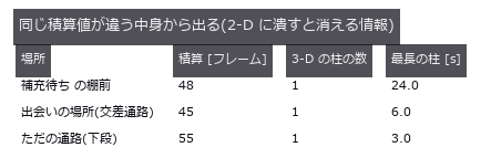
↑ The measurement ―― ヒートマップは場所を当てるが、「1 人が長く待った」と「何人も短く止まった」を分けない。 (figure labels are in Japanese; the numbers are the same)
py -3.11 examples/poc_warehouse_flow.py
Source: examples/poc_warehouse_flow.py
Ops used (notes): esdf · face_areas · mesh_volume · occupancy_grid · render_volume_projection · vol_dilate · vol_erode · vol_label · vol_opening_ball · vol_region_props
92. The Arrival-Time Surface as an Isosurface in (x, y, t)
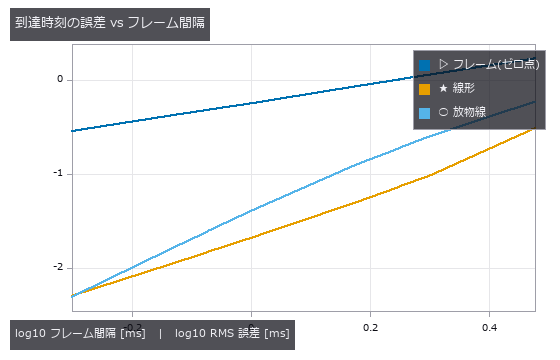
↑ The Arrival-Time Surface as an Isosurface in (x, y, t) ―― The arrival-time surface of wavefronts spreading from point sources, extracted as an isosurface of the (x, y, t) volume. The null (first frame above threshold) is biased by Δt/2, which more frames cannot remove; linear sub-frame interpolation is 27x better (0.0209 ms). Parabolic interpolation loses to linear, and linear is at its best (a 3.8x margin) when the threshold sits at the Gaussian’s inflection point θ = 0.6065.
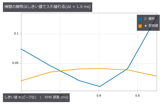
↑ The measurement ―― 変曲点 θ=0.6065 では線形が 3.8 倍勝ち、θ=0.2 では放物線が 3.6 倍勝つ。交点は θ≈0.35 と θ≈0.75。 (figure labels are in Japanese; the numbers are the same)
py -3.11 examples/poc_xyt_event_surface.py
Source: examples/poc_xyt_event_surface.py
Ops used (notes): vertex_normals · vol_edge_probe
The Geometry and Calibration Wing — A Small Residual Is Not Proof of Correctness
Reprojection error in camera calibration, seam mismatch in a panorama, residual in point-cloud registration: all are read as ‘smaller is better’. The three exhibits here, with ground truth in hand, show where that reading fails.
Reprojection RMS of 0.0688–0.0690 px alongside focal-length errors of 0.026–7.334 %. Adjacent seams at 0.12 px while the single closing seam opens by 1.5 px. Spheres and cylinders converging to the same residual with an arbitrary pose. Least squares drives the residual down to the noise; whether it lands on the truth is a separate question.
A trap in the measuring procedure itself is kept on display: fix one point cloud and sweep only the pose, and you still have a sample of one — the random seed alone produced both ‘0 % quadrant errors’ and ‘100 %’. About the only absolute quantity measurable without ground truth is the loop-closure error of a full 360-degree sweep.
93. A Reprojection Error of 0.05 px Guarantees Nothing
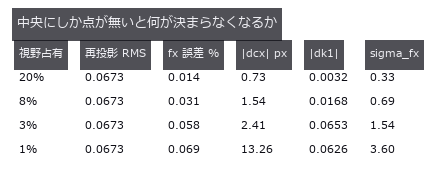
↑ A Reprojection Error of 0.05 px Guarantees Nothing ―― Grid points projected with known intrinsics and poses, re-calibrated, and the error split by component. With the board tilted 32 / 8 / 2 degrees the reprojection RMS spans 0.0688 to 0.0690 px (ratio 1.00) while the focal-length error spans 0.026 to 7.334 % (281x). With a distorting camera the degeneracy gate never fires, and the non-linear optimiser returns an answer even for a fronto-parallel board.
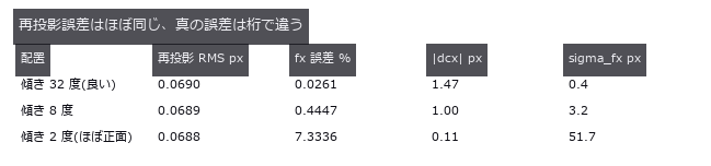
↑ The measurement ―― RMS は 1.00 倍しか動かないのに fx 誤差は 281 倍動く。配置の良し悪しを映すのは sigma_fx のほう。 (figure labels are in Japanese; the numbers are the same)
py -3.11 examples/poc_camera_calibration.py
Source: examples/poc_camera_calibration.py
Ops used (notes): project_points · reprojection_error
94. Chain the Neighbours Together and You Cannot Get Back Where You Started
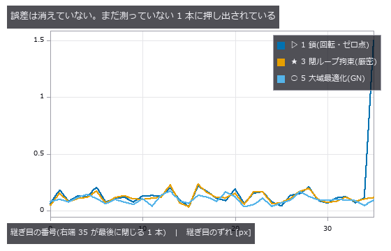
↑ Chain the Neighbours Together and You Cannot Get Back Where You Started ―― 36 frames cut from a cylindrical panorama by a known rotation sequence and chained pairwise around a full turn. Adjacent seams agree to 0.12 px, yet the one closing seam opens by 1.5 px (13x). The buried bundle_adjust_mosaic did not beat the chain (30 of 36 frames were left as the identity); the worst pose error goes from 1.65 px for the chain to 0.56 px with global optimisation.

↑ The measurement ―― 系 2(等分)は閉ループ誤差を下げるのに姿勢はかえって悪化する。新しい観測を足さずに効くのは系 3。 (figure labels are in Japanese; the numbers are the same)
py -3.11 examples/poc_panorama_drift.py
Source: examples/poc_panorama_drift.py
Ops used (notes): pose_error · warp_by_plane
95. Measuring on a Real Stereo Photograph — Three Stumbles Synthesis Never Produces
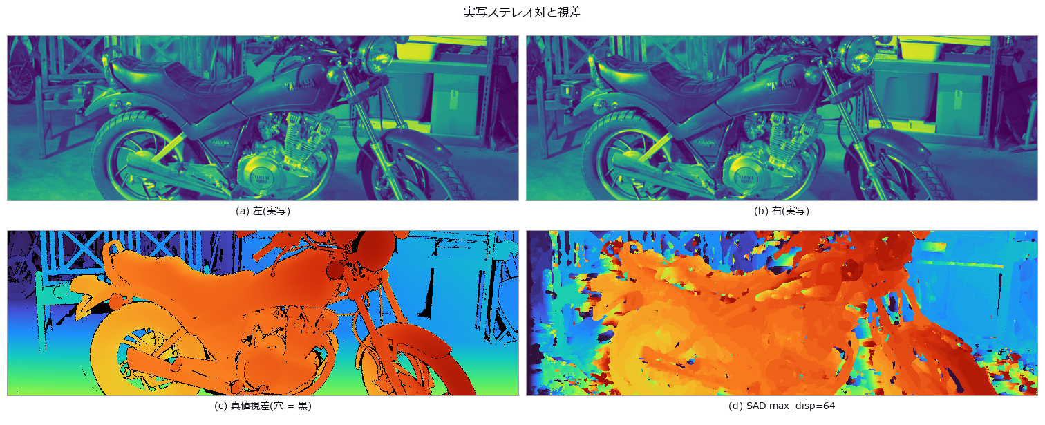
↑ Measuring on a Real Stereo Photograph — Three Stumbles Synthesis Never Produces ―― The first exhibit in this museum measured on a real photograph (Middlebury 2014 motorcycle, with ground-truth disparity). The distributor’s own note says the holes in the truth are NaN; they are +inf, so np.nanmedian reports a median disparity of 44.97 px instead of 42.55 px, while fill_disparity and apply_cmap — which test with isfinite — handle them correctly. The default max_disp=16 scores bad2 95.06 %: any search range below the true maximum of 59.91 px loses the whole foreground, so the cliff sits between 48 and 64, which geometry predicts before any measurement. Against a 94.04 % null, SGM scores 15.81 %, and discarding the least confident 40 % takes it to 6.80 %. Converting to metric depth bends the scene: depth_from_disparity had no principal-point offset, and ignoring the real doffs of 31.086 px puts points 1.519 to 5.243 times too far — no single scale repairs it, since the best factor of 0.3733 still leaves 958.3 mm RMS over a 2889 mm range, pushing far surfaces +1676 mm out and pulling near ones -926 mm in. The argument was added here, and it reproduces the closed form exactly.

↑ The measurement ―― 下位 4 割を捨てると bad2 は 26.75 % -> 6.80 %。 (figure labels are in Japanese; the numbers are the same)
py -3.11 examples/poc_real_stereo_depth.py
Source: examples/poc_real_stereo_depth.py
96. The Convergence Basin of Point-Cloud Registration — How Far Off Can the Initial Pose Be?
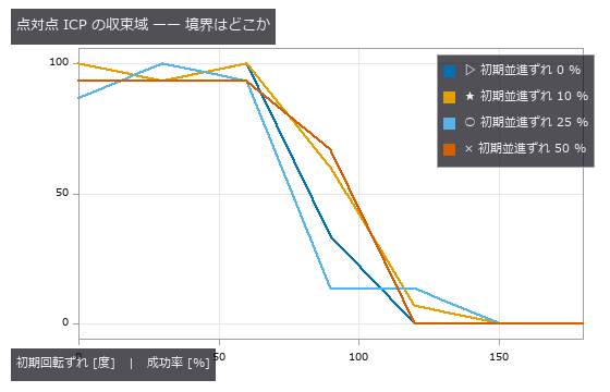
↑ The Convergence Basin of Point-Cloud Registration — How Far Off Can the Initial Pose Be? ―― ICP success rate contoured against the initial pose error, with the point cloud re-sampled on every trial. With no translation offset, success drops below 50 % at 90 degrees for point-to-point and 120 degrees for point-to-plane. Spheres and cylinders converge to the same residual with an arbitrary pose; with the global method all 16 of 16 trials appear converged and the pose is wrong — undetectable from the residual.
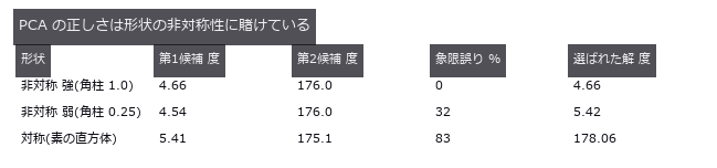
↑ The measurement ―― 非対称性が消えると 4 候補が形として区別できず、選択が崩れる(選ばれた解が第 1 候補から離れる)。 (figure labels are in Japanese; the numbers are the same)
py -3.11 examples/poc_registration_basin.py
Source: examples/poc_registration_basin.py
Ops used (notes): estimate_normals · farthest_point_sampling · rmse
97. Which Quantities Really Survive a Rotation — Auditing Invariance on a Real Coin
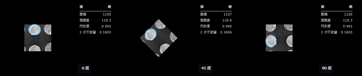
↑ Which Quantities Really Survive a Rotation — Auditing Invariance on a Real Coin ―― Shape features are routinely called rotation-invariant, but the pixel grid is not invariant under rotation, so the claim usually breaks at a helper — how the boundary is counted, how the image is interpolated, where the threshold lands. A real photograph (scikit-image coins, Greek coins from Pompeii, British Museum) is turned through a full circle in 5-degree steps and the wobble is split into three arms: A rotate the greyscale and re-threshold (what people actually do), B rotate the 0-degree binary mask with nearest neighbour (re-rasterisation only), C multiples of 90 degrees via np.rot90 (exact). The rotation itself is done with scipy, not with fullseye — measuring your own invariance with your own rotation hides errors that lean the same way. Arm C is exactly 0.00 % for all seven quantities: the measurements carry no orientation bias at all, so every bit of the wobble is the cost of re-laying the boundary on the grid. The prediction was wrong: rotating the *binary mask turns out to be far worse than interpolating the grey — perimeter 2.52 % (A) vs 9.47 % (B), circularity 4.82 % vs 20.45 %. Nearest-neighbour rotation re-lays a staircase; interpolating the grey re-derives the boundary from the underlying continuous signal. Rotate the greyscale, never the mask. A synthetic square anchors the closed form: the 4-connected staircase perimeter of a square rotated 45 degrees is bounded by 4L → 4L√2 (+41.4 %), but the measured swing is 7.91 % because regionprops applies a Crofton-style correction — the closed form is a ceiling, not a prediction. Finally, check the denominator: Hu[1] is ~0 for a near-circular blob (3.9e-04), so its 29.6 % relative spread means nothing at all.*
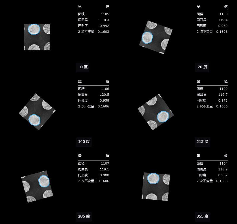
↑ The measurement ―― 実写の硬貨を 5 度ずつ 1 周。地がモノクロなので輪郭は彩度のある色で描いている(灰色には彩度が無いので、どの階調とも色相で区別がつく)。右の表の数字がどれだけ揺れるかが見える。 (figure labels are in Japanese; the numbers are the same)
py -3.11 examples/poc_rotation_invariance_audit.py
Source: examples/poc_rotation_invariance_audit.py
Ops used (notes): annotate_outline · annotate_table · blob_features · blob_label · circularity · eccentricity · moments_region_2nd_invar · moments_region_central_invar · text_box
The Colour and Separation Wing — There Is No Method That Works, Only Conditions Under Which One Does
Estimating the illuminant to restore colour, peeling the layers of a painting with multiple wavelengths, separating specular reflection with polarisation. The three exhibits here synthesise linear radiance from known spectral reflectances, known illuminants and the Fresnel equations, then compare the separation against that truth.
The conclusion in every case was that the failure axes are orthogonal. Max-RGB is best when a white patch is present and gets 8x worse when the single brightest patch is removed; grey-world shrugs off saturation but loses once chromatic content exceeds 20 %; under a reference illuminant every method loses to doing nothing; adding bands does not win, adding near-infrared does.
The shared warning is to convert to linear radiance before calling anything. Pass sRGB-gamma values and no exception is raised; the separation simply degrades in silence. Failure without an exception is the most common pattern in the whole museum.
98. Peeling Layers With Many Wavelengths — Underdrawing, Ground, Glaze and Fading, Truth in Hand
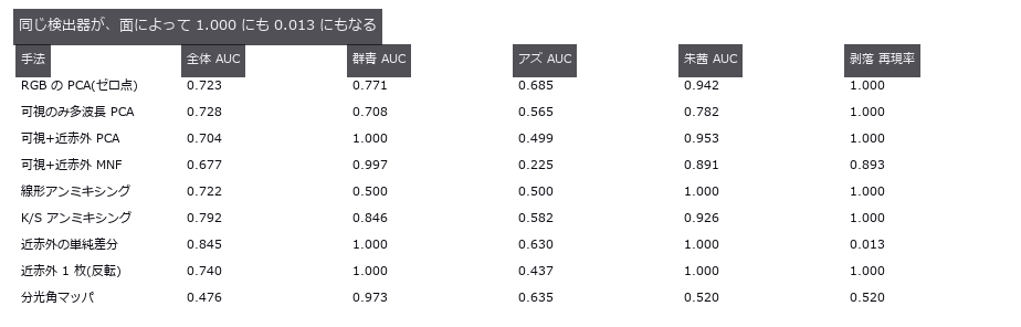
↑ Peeling Layers With Many Wavelengths — Underdrawing, Ground, Glaze and Fading, Truth in Hand ―― A spectral cube of ground, underdrawing, glaze and fading stacked in layers, then unmixed. Splitting the visible range into 16 bands does no better than RGB (recall 0.118 versus 0.119); what won was adding near-infrared. The same detector scores an AUC of 1.000 on ultramarine, 0.630 on azurite and 0.013 on losses — averaged, all of that vanishes. Restoring the unfaded colour barely beat the null, ΔE00 16.79 → 16.46.
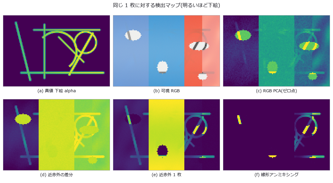
↑ The measurement ―― 近赤外の差分は剥落部(楕円)で消え、近赤外 1 枚は面ごとに水準が違う。塗り分けは 1–99 分位でクリップした表示のみ。 (figure labels are in Japanese; the numbers are the same)
py -3.11 examples/poc_pigment_unmixing.py
Source: examples/poc_pigment_unmixing.py
Ops used (notes): delta_e_map · linear_to_srgb · spectrum_to_srgb · threshold
99. Stripping Specular Reflection With Polarisation — Truth From the Fresnel Equations
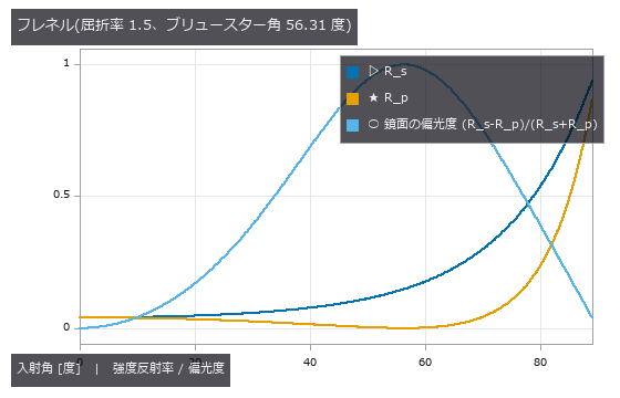
↑ Stripping Specular Reflection With Polarisation — Truth From the Fresnel Equations ―― Diffuse and specular components synthesised as s/p terms with the degree of polarisation from the Fresnel equations, and the separation scored against them. At 20 degrees of incidence the polarisation method wins by only 1.2x. The diffuse error matches the closed form R_p·E exactly and vanishes at the Brewster angle of 56.31 degrees — the diffuse term of polarization_separate is systematically high by that amount.
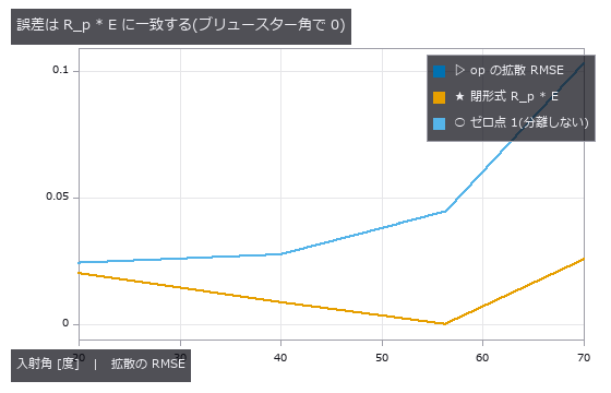
↑ The measurement ―― 実測と閉形式が重なる。70 度の絶対誤差は 20 度より悪いのに、ゼロ点比では 70 度が最良 —— 最適角は評価軸で割れる。 (figure labels are in Japanese; the numbers are the same)
py -3.11 examples/poc_polarization_specular.py
Source: examples/poc_polarization_specular.py
Ops used (notes): fresnel_reflectance · polarization_dolp_map · polarization_render · polarization_separate · polarization_stokes · rmse
100. Separating a Real Immunostain by Colour — The Watchdog Was Blind to Exactly the Error It Should Catch
↑ Separating a Real Immunostain by Colour — The Watchdog Was Blind to Exactly the Error It Should Catch ―― Colour deconvolution of a real immunostain (haematoxylin plus DAB). On synthetic data it separates perfectly — recompose one stain at unit concentration, solve again, and recovery is 1.0000 with 0.0000 crosstalk — so anyone looking only at synthesis concludes the problem is solved. On the real slide the haematoxylin concentration runs down to -4.446 and 11.51 % of pixels are negative, which is physically impossible: a negative concentration means the dye emitted light. Rotating the stain vectors within their plane by plus or minus twenty degrees moves the haematoxylin median from 0.0471 to 0.1348, a factor of 2.86, and DAB from 0.3590 to 0.1836 — while the residual channel, the quantity everyone reads as goodness of fit, stays at 0.0345 with a total spread of 3.3e-16. The geometry says why: the plane the two stains span is unchanged by a rotation inside it, so the component orthogonal to that plane cannot move. The negative fraction of the rotated stain is equally blind, fixed at 11.51 %, because its dual vector changes length but not direction. Only the partner moves, from 0.00 % at minus twenty degrees to 30.38 % at plus twenty: the watchdog has to watch the other stain, not itself, and being monotone it bounds the error from one side only. The round trip through recompose closes to 1e-06, which refutes none of this.
↑ The measurement ―― H の中央値は 0.0656 -> 0.1348。残差の絶対中央値は 0.0345 のまま。 (figure labels are in Japanese; the numbers are the same)
py -3.11 examples/poc_real_stain_unmix.py
Source: examples/poc_real_stain_unmix.py
101. Colour Constancy (White Balance) — No Method Works, Only Conditions Do
↑ Colour Constancy (White Balance) — No Method Works, Only Conditions Do ―― Linear RGB synthesised from 24 known spectral reflectances and known illuminants, with illuminant estimation scored by recovery angular error. Max-RGB is best at a median of 1.06 degrees over 11 illuminants, but removing the single brightest patch takes it to 8.45 degrees, and tripling exposure to saturate 43 % of pixels takes it to 13.61 degrees, identical to doing nothing. Even a diagonal correction with the true illuminant leaves a mean ΔE00 of 5.07 at 2500 K.
↑ The measurement ―― 灰色世界はゼロ点(何もしない)の線を 0.1〜0.2 の間で上抜けする = そこから先は回すだけ損。白パッチ法には崖が無い。 (figure labels are in Japanese; the numbers are the same)
py -3.11 examples/poc_white_balance.py
Source: examples/poc_white_balance.py
Ops used (notes): delta_e_map · gauss_filter · illuminant_from_dichromatic_planes · laplace · linear_to_srgb · mean_image · prewitt_amp · roberts · sobel_amp · spectrum_to_srgb
The Forensics and Documents Wing — One Successful Image Is Not Evidence
Forgery detection and document rectification. Both tend to be presented through ‘the one image where it was found’ or ‘the one page that came out straight’. The two exhibits here fix the paste location and quality, the homography and the lighting themselves, then score with a per-pixel ROC and pixel-level geometric error.
The forgery exhibit is on the detection (defensive) side. Forgeries are generated only because scoring a detector needs ground truth, and the generator is kept to the crudest form possible. What the exhibit shows most strongly is the fact that works against the detector: one press of the save button weakens every cue.
The document exhibit puts a number on a hole: two functions with the same name and different models can be swapped without an exception, returning a plausible picture with the keystone still in it. Shadow removal has no free lunch; the flatter the paper, the more of the faint text disappears.
102. Straightening a Hand-Held Document Photo — Keystone Correction and Shadow Removal Against Ground Truth
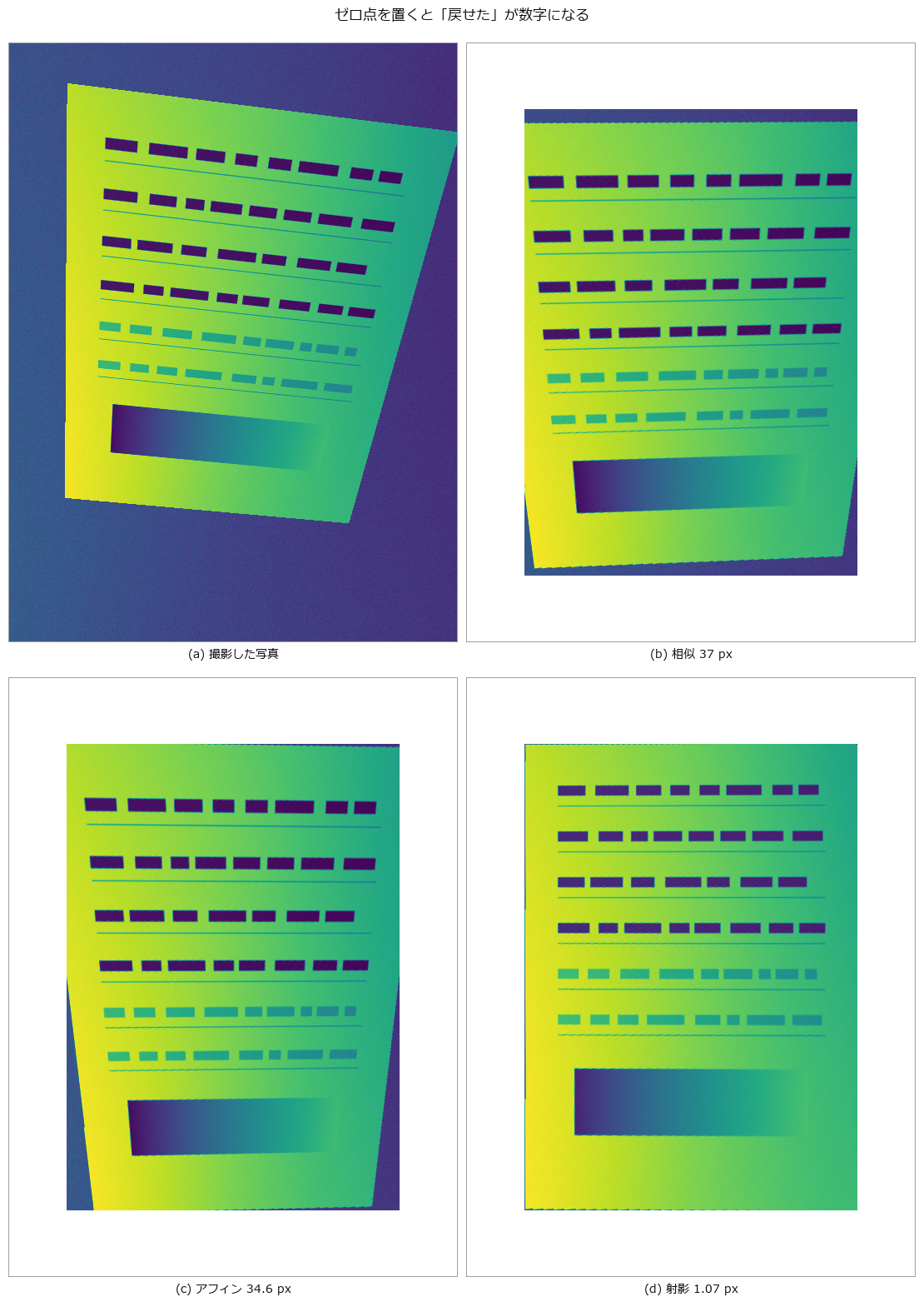
↑ Straightening a Hand-Held Document Photo — Keystone Correction and Shadow Removal Against Ground Truth ―― A document imaged under a known homography and lighting, rectified, and scored by corner and grid error in pixels. The estimate reaches a grid RMS of 1.070 px (doing nothing: 37.376 px), but swapping in the same-named function with a different model (affine) is 32x worse and raises no exception. Shadow strength 0.45 gives a corner RMS of 5.72 px; 0.55 gives 65.10 px — a cliff.
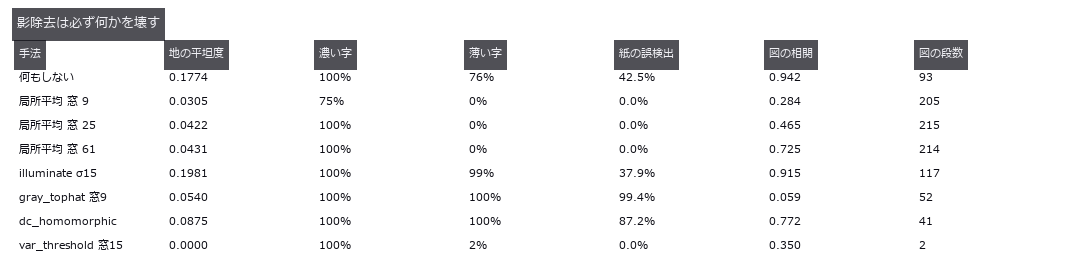
↑ The measurement ―― 平坦・薄字・誤検出なしを同時に満たす行は 1 つも無い。窓 9 が fs.op で届く上限、窓 61 は自前。図の階調は真値で 217 段。 (figure labels are in Japanese; the numbers are the same)
py -3.11 examples/poc_document_scan.py
Source: examples/poc_document_scan.py
Ops used (notes): corner_response · dc_homomorphic · fill_holes · gauss_filter · get_region_contour · gray_tophat · illuminate · mean_image · opening_circle · otsu · project_points · reflect · select_largest · sobel_dir · var_threshold
103. Forgery Detection as an ROC — Not the One Image Found, but Detection at a Fixed False-Positive Rate

↑ Forgery Detection as an ROC — Not the One Image Found, but Detection at a Fixed False-Positive Rate ―― Ten forgeries made by pasting a JPEG q60 patch onto a q92 background and saving at q95, scored with a per-pixel ROC. ELA’s single number points the opposite way from the textbook (paste / background = 0.58x), and an untouched image still yields an AUC of 0.797 from position bias alone. The ghost-valley depth reaches an AUC of 0.997, which falls to 0.975 after one whole-image recompression at q75.
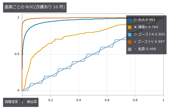
↑ The measurement ―― 凡例の数字は AUC。乱数が対角線に乗ることで測り方に偏りが無いと言える。ゴーストA は乱数と重なる。 (figure labels are in Japanese; the numbers are the same)
py -3.11 examples/poc_forensics_roc.py
Source: examples/poc_forensics_roc.py
Ops used (notes): copy_move_regions · error_level_map · jpeg_ghost_map · jpeg_ghost_quality · noise_inconsistency_map · reflect
104. Craquelure networks — of three indicators, only junction degree breaks under imaging conditions
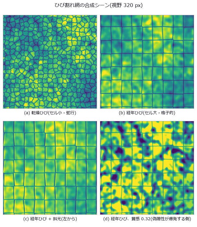
↑ Craquelure networks — of three indicators, only junction degree breaks under imaging conditions ―― A Voronoi crack network is drawn in closed form for two ground-truth types — drying cracks (small tortuous cells) and age cracks (large grid-like cells) — with paint blotches, varnish gloss, raking light, blur and noise, then measured with a ridge op → skeleton → junction chain. Truth separates the types on all three indicators (cell diameter 18.0 vs 45.2 px, straightness 0.960 vs 1.000, degree-4 fraction 0.20 vs 0.83), yet the age type’s degree-4 fraction drifts toward the drying value under texture (0.87 → 0.64) and raking light (0.70) while diameter and straightness stay put. Both predicted cliffs failed to appear: recall is still 0.696 at 0.15 px width and false positives only 0.382 at texture contrast 0.64. Raking light widens cracks one-sidedly by +0.37 px and shifts the centreline 0.75 px toward the light.
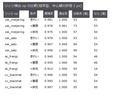
↑ The measurement ―― Frangi は分岐点で応答が落ち、斜光でセルが崩れる。 (figure labels are in Japanese; the numbers are the same)
py -3.11 examples/poc_fresco_craquelure.py
Source: examples/poc_fresco_craquelure.py
Ops used (notes): blob_features · blob_label · blob_overlay · cv_blackhat · distance_transform · hx_split_skeleton_region · hysteresis_threshold · junctions_skeleton · otsu · pruning · r2_endpoints_skeleton · sk_area_opening · sk_frangi · sk_otsu · skeleton · threshold · xsk_meijering · xsk_sato
105. Camera Fingerprints (PRNU): Which Camera Took This? — The Fingerprint Grows With Frame Count and Dies at the Save Button
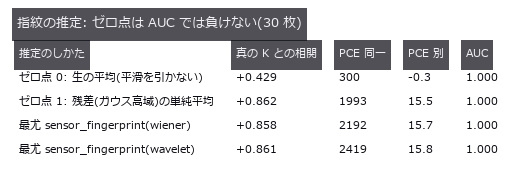
↑ Camera Fingerprints (PRNU): Which Camera Took This? — The Fingerprint Grows With Frame Count and Dies at the Save Button ―― Two virtual cameras carry a fixed sensitivity pattern K; the fingerprint is estimated from 30 residuals and matched. Under clean conditions the same camera scores a median PCE of 2192 against 15.7 for the other (AUC 1.000), but JPEG-like quantisation at quality 50 cuts PCE to 3.6 % and a 0.5x downscale to 1.5 % — and what killed it was the residual extractor, not the geometry. A camera with K = 0 still yields a ‘fingerprint’ with PCE 1706 if the same background is shot 30 times: the scene turns into a fingerprint.
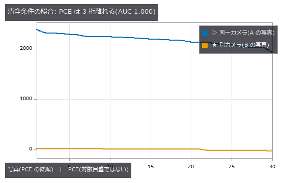
↑ The measurement ―― 別カメラのピークは毎回別の位置に立つ((0,0) は 0/30)。 (figure labels are in Japanese; the numbers are the same)
py -3.11 examples/poc_prnu_camera_fingerprint.py
Source: examples/poc_prnu_camera_fingerprint.py
Ops used (notes): aug_jpeg_blocks · evidence_quantile · fingerprint_correlate · gauss_image · median_image · null_distribution · reflect · sensor_fingerprint · sk_nlm · sk_tv · sk_wavelet · xsp_dct_denoise · xsp_wiener
The 3-D Shape Wing — Align First, and the Alignment Eats the Defect
Work on point clouds and meshes differs from 2-D work in one decisive way: a pose-alignment step comes before the measurement. That step rotates the shape into whatever orientation makes the discrepancy smallest, so the larger the defect, the more of it the alignment absorbs, leaving a small residual and a part that looks in tolerance. The exhibits in this room try to count what the alignment ate.
Every ground truth here is written as a formula. Solids are built from analytic surfaces combined with boolean operations, chosen so that volume, surface area, wall thickness and curvature are known in closed form. Deformations are known fields (a local dent, a warp, a constant wear along the surface normal), poses are known rotations and translations, and the scan is a uniform sample of the surface with a known density, noise level and occlusion pattern. That is what makes it possible to hold the alignment error and the shape error apart.
The pitfalls specific to 3-D also get counted separately here. A nearest-neighbour distance is biased upward whenever there is noise, because it only ever counts one side. Normal signs are decided by whatever helper computed them. Changing the point density changes the scale of the distance itself. A symmetric shape has no unique pose. Each of these disappears the moment the numbers are folded into one.
106. Battery cell degradation by CT — the swelling shows outside, the cause stays inside
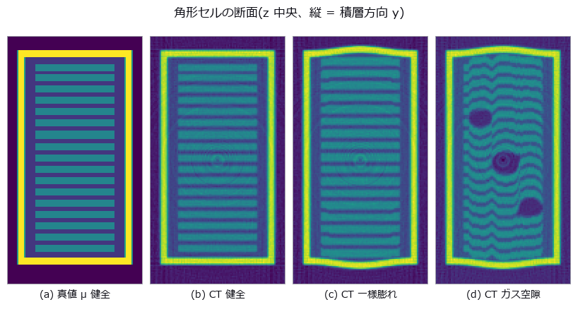
↑ Battery cell degradation by CT — the swelling shows outside, the cause stays inside ―― A prismatic lithium-ion cell — stacked electrodes inside an aluminium can — is built with ground truth, degraded by known fields (uniform swelling, local swelling, inter-layer gas voids, electrode misalignment), and then imaged for real: forward projection, beam hardening, photon noise and FBP reconstruction. Only 29.4 % of a 10 % electrode swelling reaches the outside, and a caliper across the centre reads 3.6 times the volume-equivalent mean (+0.235 vs +0.066 mm). Three cells tuned to the same external bulge differ by 0.000 mm in can height yet separate internally (void fraction 0.00 vs 5.20 %, layer flatness 0.0156 vs 0.0784 mm), and the resolution cliff for those internal numbers is set by the 0.120 mm inter-layer gap, not the 0.200 mm electrode — voxel/thickness = 0.30, where the sampling-theorem prediction said 0.80.
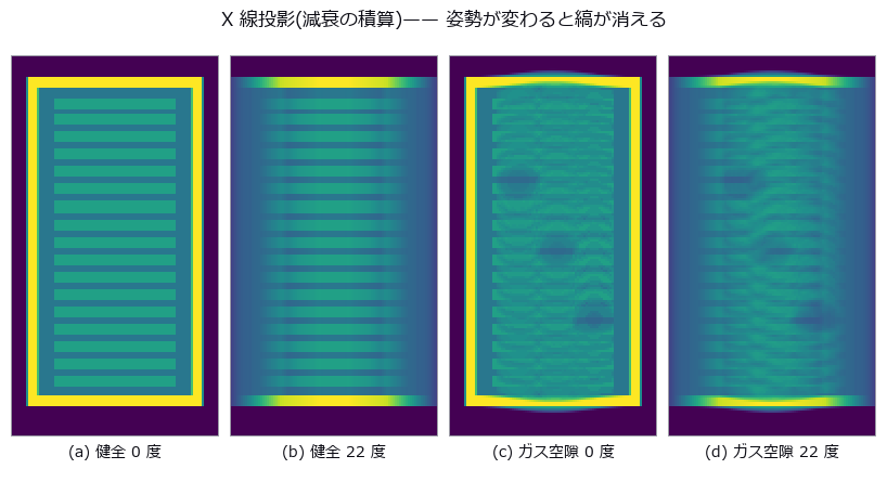
↑ The measurement ―― 真正面(0 度)なら空隙の影までは見える。ただし奥行きに積算されているので厚みも深さも出ない。22 度傾けると層の縞そのものが重なって消える —— 投影では姿勢が結果を決めてしまう。だから断層に落とす。 (figure labels are in Japanese; the numbers are the same)
py -3.11 examples/poc_battery_ct_degradation.py
Source: examples/poc_battery_ct_degradation.py
Ops used (notes): beam_hardening_apply · box_sdf · fbp_volume · grid_coords · plane_sdf · projection_angles · radon_volume · render_volume_projection · ring_artifact_apply · sdf_intersect · sdf_subtract · sdf_to_occupancy · sdf_union · vol_bounding_box · vol_edge_probe · vol_fft_lowpass · vol_label · vol_profile_line · vol_region_props · vol_resize · vol_wall_thickness
107. Fusing two sensors into a bird’s-eye grid — a calibration that passes in pixels turns into metres at range

↑ Fusing two sensors into a bird’s-eye grid — a calibration that passes in pixels turns into metres at range ―― An analytic street scene (a tall lead truck, plus two distant cars each hidden in the other sensor’s shadow) is fused from a left-mirror LiDAR and a right-mirror depth camera into one bird’s-eye grid, then swept over rotation, translation and timing errors in the extrinsics. Fusion reaches an occupancy IoU of 0.7033 against 0.5417 for the best single sensor — and every bit of that gain comes from complementary visibility, not accuracy. One pixel of reprojection error becomes 0.083 m at 22 m; the cliff is set by the object width, not the 0.2 m cell (IoU drops only 5.8 % when 68 % of the points have already crossed a cell); by 3 deg of yaw the fusion has fallen below the single sensor.

↑ The measurement ―― 横に 1.80 m 離した 2 センサの「自由と言い切れた領域」。青い帯が LiDAR にしか見えない所、橙の帯がカメラにしか見えない所、灰色は両方。白は真値の障害物。22 m の 2 台は互いの影に 1 台ずつ入っている。 (figure labels are in Japanese; the numbers are the same)
py -3.11 examples/poc_bev_sensor_fusion.py
Source: examples/poc_bev_sensor_fusion.py
Ops used (notes): box_sdf · closing_circle · depth_to_points · esdf · fill_up · fuse · grid_coords · occupancy_grid · project_points · sdf_to_occupancy · sdf_union · voxel_grid_downsample · voxel_iou
108. CAD-to-scan deviation inspection — the fit absorbs the defect and invents a dent
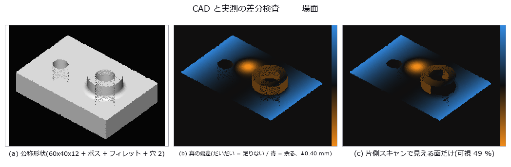
↑ CAD-to-scan deviation inspection — the fit absorbs the defect and invents a dent ―― An analytic machined part carries a known local dent, a bow and a wear band, all applied as exact displacements along the surface normal, and the scan is synthesized with a known pose, noise and one-sided occlusion. After alignment the signed deviation and the out-of-tolerance area show that the local dent is diluted by only 3.7 %, while a 121 um dent appears at the centre of the part where the truth is just 1.2 um (closed form predicts -120 um). What survives depends on how much the defect resembles the six rigid-body degrees of freedom; along the edges the nearest neighbour jumps to the adjacent face, producing 66.5 mm^2 of false out-of-tolerance area even in a defect-free control.
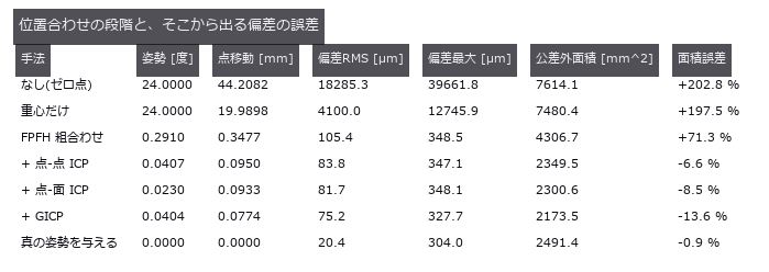
↑ The measurement ―― 真の姿勢を与えた最終行が推定器そのものの床。点-面 ICP との差は姿勢ではなく datum の取り方の差。 (figure labels are in Japanese; the numbers are the same)
py -3.11 examples/poc_cad_scan_deviation.py
Source: examples/poc_cad_scan_deviation.py
Ops used (notes): box_sdf · chamfer_distance · esdf · estimate_normals · estimate_oriented_normals · face_areas · gicp · hausdorff_distance · icp_point2plane · icp_point2point_3d · query_distance · register_fpfh · sphere_sdf · voxel_grid_downsample
109. Crop leaf area from above — folded by projection before it is ever hidden

↑ Crop leaf area from above — folded by projection before it is ever hidden ―― A maize canopy built from analytic leaf surfaces (one-sided area pi/4·L·W, leaf angle and projection coefficient both closed-form) is viewed through an exact nadir z-buffer to measure cover, occlusion and leaf angle. Inverting cover with Beer-Lambert underestimates a true leaf area index of 4.85 by 52.2 % even with the exact extinction coefficient, and stalls just above the ceiling of 2.26 predicted from two-scale clumping (measured 2.70). Occlusion changes nadir cover by not one bit; what breaks the estimate is the folding of projection — an average of 3.49 leaves cover a cell yet are counted once — and quadrupling point density buys only +1.92 in the largest resolvable index.

↑ The measurement ―― 閉形式 2 pi r h + 4 pi r^2 / pi r^2 h + 4/3 pi r^3 と比べる。2 値化を挟むと面積だけが一方向に膨らむ。 (figure labels are in Japanese; the numbers are the same)
py -3.11 examples/poc_crop_phenotyping.py
Source: examples/poc_crop_phenotyping.py
Ops used (notes): boundary_vertices · capsule_sdf · dem_slope · estimate_normals · face_areas · face_normals · grid_coords · mesh_area · mesh_sample_points · mesh_volume · occupancy_grid · plane_segmentation · render_volume_projection · sdf_to_occupancy
110. Collapsing joint voids into one number — what the number drops is the shape that matters

↑ Collapsing joint voids into one number — what the number drops is the shape that matters ―― A synthetic die-attach bond line carries five void populations whose volume fraction is held exactly at 3.000 % while only their depth, shape and proximity change, re-imaged as an X-ray CT with a PSF, noise and beam-hardening cupping. The naive zero point — threshold, then report void fraction — separates the five conditions by only 0.17 points (2.46 to 2.63 %), yet the interface area shadowed by flat voids is 2.09x that of volume-matched spheres (14.49 vs 6.92 %) and the largest cluster spans 13.1x further when the voids are chained (80.0 vs 6.1 %). The predicted cliff never arrives: at 60 um voxels the void fraction still reads 3.21 % (it only wobbles by 1.36 points with the grid phase), while flatness becomes unmeasurable and the interface-deficit metric drops from 14.16 to 9.78 % — the degradation runs toward ‘pass’, which is the worst possible direction.

↑ The measurement ―― 疑似カラーはラベル番号を並べ替えたもの。側面図で界面(上端)に貼りついているのが見える。 (figure labels are in Japanese; the numbers are the same)
py -3.11 examples/poc_ct_void_morphology.py
Source: examples/poc_ct_void_morphology.py
Ops used (notes): boundary_vertices · box_sdf · cylinder_sdf · esdf · face_areas · mesh_volume · morph_dilate3d · plane_sdf · query_distance · sdf_union · sphere_sdf · vol_boundary_points · vol_gaussian_psf · voxel_to_mips
111. Manufacturability from geometry alone — faces that sit on the threshold flip when you smooth them
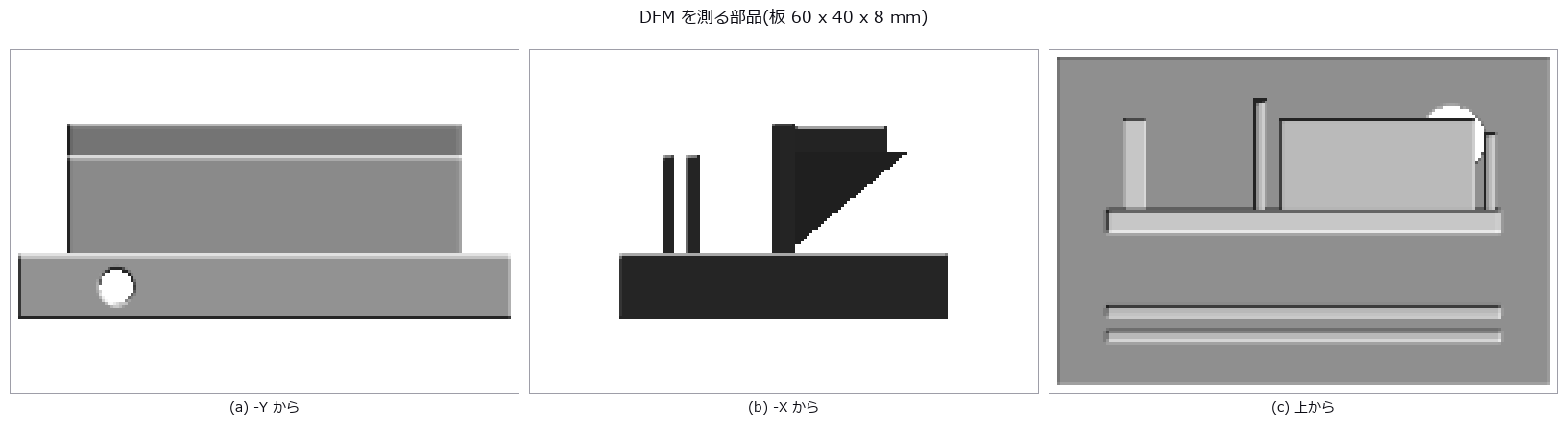
↑ Manufacturability from geometry alone — faces that sit on the threshold flip when you smooth them ―― A synthetic part with known design values (thin walls, a slot, ribs near 45 deg, holes) is voxelised, then wall thickness, support area and tool clearance are measured. Across the 45 deg threshold the support area jumps 185.22 -> 576.10 mm^2 — 3.11x for 0.2 deg — and that step vanishes entirely when the isosurface is taken from a distance field, and loses 12 % under smoothing. Thickness collapses onto a 2-voxel lattice (the inscribed sphere does not help), and clearance errors go both ways: at 0.500 mm voxels the slot appears 2.000 mm wide and admits a tool that does not fit.
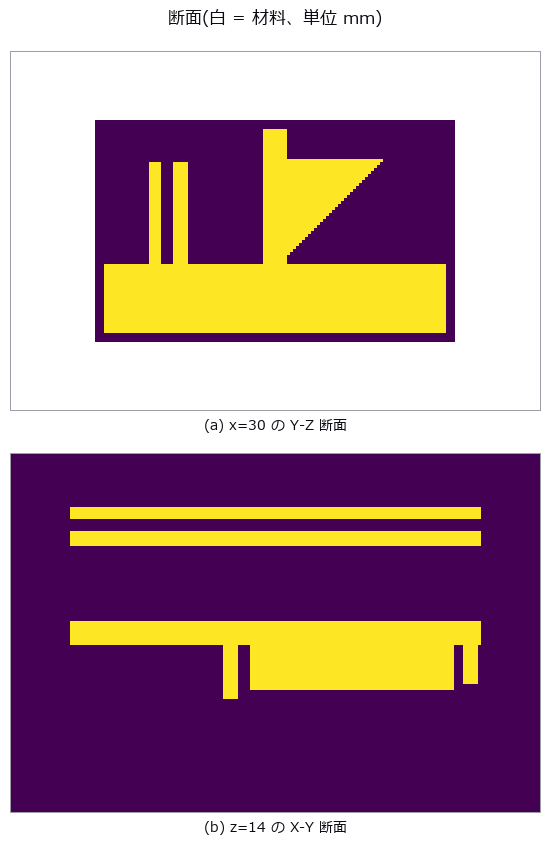
↑ The measurement ―― 上: 左端の 2 本が薄壁(1.500 mm)とそのあいだのスロット(1.500 mm)、右の三角が補強。下: リブと薄壁の footprint。 (figure labels are in Japanese; the numbers are the same)
py -3.11 examples/poc_dfm_thickness_overhang.py
Source: examples/poc_dfm_thickness_overhang.py
Ops used (notes): box_sdf · esdf · face_areas · face_normals · grid_coords · morph_erode3d · render_shaded · sdf_intersect · sdf_subtract · sdf_to_occupancy · sdf_union · vol_wall_thickness · voxel_to_mesh
112. Earthwork on a slope — align first and the scar gets shallower
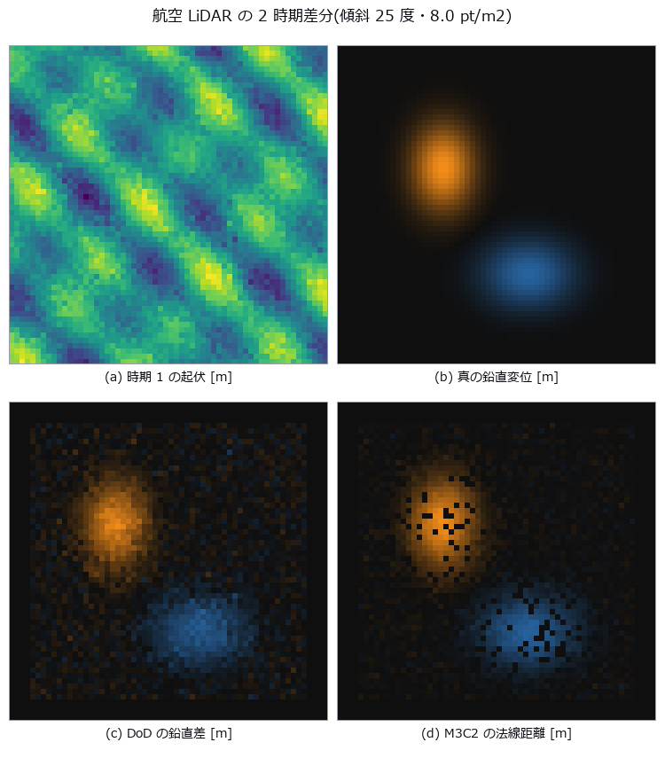
↑ Earthwork on a slope — align first and the scar gets shallower ―― A synthetic slope carries an excavation and a deposit of known volume; two epochs of airborne points are differenced both vertically (DoD) and along the local surface normal (M3C2). The expected “cos-θ shrinkage on a slope” never appears — integrating vertical differences over horizontal area cancels the cosine, and the excavated volume stays within -0.011 % from 0 to 40 degrees. What breaks is the registration: when the changed area covers 33 % of the scene, ICP absorbs the change itself and the net volume collapses from a true -30.4 m3 to -3.8 m3, while a no-change control alone already fabricates 83.8 m3 of phantom excavation.
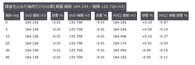
↑ The measurement ―― 傾斜を 0 から 40 度まで振っても体積の誤差に傾向が無い。cos は積分で約分する。 (figure labels are in Japanese; the numbers are the same)
py -3.11 examples/poc_lidar_terrain_change.py
Source: examples/poc_lidar_terrain_change.py
Ops used (notes): chamfer_distance · estimate_normals · estimate_oriented_normals · fit_plane_3d · icp_point2point_3d · median · ransac_plane · voxel_grid_downsample
113. Weighing an Animal from Silhouettes — The Error You Can Buy Down, and the One You Cannot
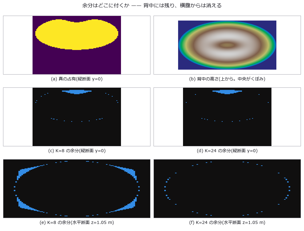
↑ Weighing an Animal from Silhouettes — The Error You Can Buy Down, and the One You Cannot ―― Estimate an animal’s volume from the intersection of multi-view silhouettes (the visual hull) and convert it to weight. A visual hull is always an upper bound, so the question is not whether it is good but that it is always high. The closed form corrected the field rule of thumb: K cameras do not give a K-gon. Under parallel projection each camera contributes two support lines perpendicular to its line of sight, and two opposing cameras contribute the same pair, so the number of distinct tangents is K for even K and 2K for odd K. Three cameras and six cameras are therefore geometrically identical (closed form 1.16772 both times, the measured 0.013 difference being discretisation only), half of an even rig is wasted, and 13 cameras (1.03056) beat 16 (1.04768). Requiring 2 % on weight needs 13 cameras if odd counts are allowed and 24 if not — the naive circular reading of (K/pi)tan(pi/K) says 13, so a team building an even-numbered rig is short by 11. Against the exact ellipse (a/b = 2.76) the measurements sit just above the closed form at every K, confirming it as a lower bound. The centre of this exhibit is separating the error you can buy down from the one you cannot: the phantom between the legs falls from 7.13 % to 1.37 % going from 4 to 48 cameras, while the hollow of the back falls only 3.8 points (56.4 % to 52.6 %) for the same twelvefold increase, because a concavity that never reaches the outline leaves no trace in any silhouette. One pixel of segmentation error is likewise unbuyable, worth +3.21 % per pixel (23.7 kg), matching Steiner’s dV/V = (S/V)delta to a ratio of 1.04 — though the text records that two opposing effects happened to cancel there. The rulers disagree on the winner: volume-derived and allometric weight both prefer 24 cameras with a two-pixel erosion, while the height of the centroid prefers no erosion at all, since the thin legs disappear first. One prediction was wrong: a tape measure wraps the body, so the 3-D convex hull was expected to be the strong method for heart girth, but it measured +55.2 % — the hull of the whole body fills in under the belly and drags the cross-section down to the ground. The convex hull of a section and the section of a convex hull are not the same object. A tooling hole was found and closed on the way: the OpenCV-convention pose helper that space carving requires was unreachable from every public tier, while the name look_at in the public API belonged to the OpenGL-convention version, so grabbing the wrong one returned an empty hull with no exception at all.
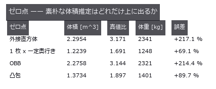
↑ The measurement ―― 真値 0.7238 m^3 / 738 kg。外接直方体と OBB は上界の中でもいちばん粗い。 (figure labels are in Japanese; the numbers are the same)
py -3.11 examples/poc_livestock_body_volume.py
Source: examples/poc_livestock_body_volume.py
Ops used (notes): carve · carve_look_at · convex_hull · erosion_circle · mesh_volume · synthesize_silhouette · vol_rle_bbox · vol_rle_centroid · vol_rle_encode · vol_rle_volume
114. Repair the mesh, then measure — the defect count clears, the quantity does not
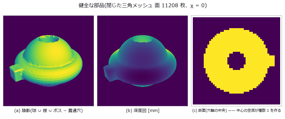
↑ Repair the mesh, then measure — the defect count clears, the quantity does not ―― A closed triangle mesh is built from the boolean union of a sphere, a torus and a box, then seeded with a known count of each defect class — holes, flipped faces, non-manifold edges, degenerate slivers, duplicated vertices and self-intersection — and tracked with both the topological counts and the volume/area. The Euler characteristic does not move at all for 5 of the 6 classes, and 6 holes plus 6 duplicated faces leave the vertex, edge, face and chi counts identical to the healthy part. Repair does not bring the quantities back: filling a 45-degree cap hole on a sphere changes the surface area by +6.868 % where the closed form predicts -2.145 % (the rim is a staircase, not a circle), and pushing just 6 vertices inward passes all three topological checks while the area is +4.414 % and the volume -0.332 % — a 13-fold disagreement.
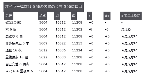
↑ The measurement ―― 健全な部品の χ は 0(種数 1)。χ=2 を合格条件にすると健全品が落ちる。最終行は打ち消し。 (figure labels are in Japanese; the numbers are the same)
py -3.11 examples/poc_mesh_quality_repair.py
Source: examples/poc_mesh_quality_repair.py
Ops used (notes): decimate_qem · face_normals · fill_holes · inertia_tensor · mesh_area · mesh_edge_lengths · mesh_edge_stats · sdf_subtract · sdf_union · vertex_curvature · vertex_normals · voxel_to_mesh
115. Pallet load utilization — one number gives voids and overhang the same value
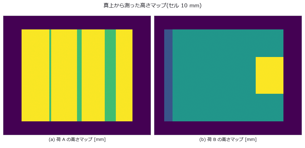
↑ Pallet load utilization — one number gives voids and overhang the same value ―― Two loads with opposite defects sit on a 1200 x 1000 mm pallet: load A hides a 400 x 400 x 420 mm cavity under a bridging layer plus 20 / 50 / 120 mm slots, while load B is solid but overhangs by 90 mm and tops out 100 mm above the 1800 mm limit. Solving the middle-layer height in closed form (995.0 mm) makes their apparent utilization identical — 62.65 % vs 62.67 %, a 0.02 pt gap — yet A’s 3.11 pt is invisible void and B’s is 2.10 pt overhang plus 0.58 pt over-height, so one load gets restacked and the other gets rejected. Treating the load as one envelope reports 113.90 % (AABB) and 166.44 % (PCA box) for load B, and the IoU between the true solid and the top-down extrusion is 0.9493 / 1.0000 — both read as ‘good agreement’. One knob, the height-map cell size, breaks the answer in two opposite directions: a slot of width w survives only as max(0, 1 - g/w) (a 20 mm slot is gone at g = 40 mm, and at g = w exactly the grid phase decides all-or-nothing — 1 alignment in 5 sees everything), while a load that overhangs by nothing acquires a false overhang of perimeter x g/2 x height that overtakes load B’s genuine 0.0450 m3 from g = 40 mm on.

↑ The measurement (figure labels are in Japanese; the numbers are the same)
py -3.11 examples/poc_pallet_load_utilization.py
Source: examples/poc_pallet_load_utilization.py
Ops used (notes): aabb · convex_hull · euclidean_cluster · inner_box3 · mesh_volume · voxel_iou
116. Pipe Wall Loss on the Unwrapped Map — The Axis You Choose Eats the Invert Corrosion
↑ Pipe Wall Loss on the Unwrapped Map — The Axis You Choose Eats the Invert Corrosion ―― A synthetic pipe carries a pit, a full-circumference thinning band, invert corrosion, a weld bead, ovality and a sagging axis, all at known depths; the in-pipe range sensor is then deliberately run off-axis before the bore is unwrapped. A 4.0 mm axis offset alone flags 44.8 % of a corrosion-free round pipe as wall loss — within 1.84 points of the geometric prediction that an offset e appears as a one-cycle sinusoid of amplitude e — and the fictitious loss volume is 149.9 times the real pit. Removing the one-cycle term removes the fiction, but 79 % of invert corrosion (the commonest defect in sewers) lives in that same harmonic, so its detection falls from 100.0 % to 34.4 %; only constraining the axis the way physics does (a straight line plus a sag) keeps both.
↑ The measurement ―― 下の帯の細くなっている所が管底腐食。 (figure labels are in Japanese; the numbers are the same)
py -3.11 examples/poc_pipe_wall_loss.py
Source: examples/poc_pipe_wall_loss.py
Ops used (notes): blob_label · blob_select · cylinder_sdf · cylinder_unwrap · esdf · polar_unwrap · ransac_cylinder · render_volume_projection · sdf_subtract · sdf_to_occupancy · spectrum · vol_wall_thickness
117. Warpage lives in the layer history — averaging the area throws the placement away
↑ Warpage lives in the layer history — averaging the area throws the placement away ―― Seven synthetic parts are sliced into layers with a known constant per-layer shrinkage strain; warpage is first predicted in closed form from the layer-area history alone, then measured with an incremental layer-birth finite-element solve. A predictor that looks only at the final shape returns exactly zero (2.712e-21), and the history-based closed form lands within 0.4 % on 4 of the 7 shapes — but the moment the area is averaged along the length, where the material sits is lost. Three parts whose layer-area histories match to the last square millimetre bow by 0.4109 / 0.3809 / 0.3271 mm (a 26 % spread), and the force peeling them off the build plate differs by 48x (11.8 vs 573.5 N), flipping the pass/fail verdict.
↑ The measurement ―― この断面の面積の列だけが、閉形式の入力になる。 (figure labels are in Japanese; the numbers are the same)
py -3.11 examples/poc_print_warpage_risk.py
Source: examples/poc_print_warpage_risk.py
Ops used (notes): blob_features · blob_label · box_sdf · grid_coords · render_volume_projection · sdf_to_occupancy · sdf_union · text_box
118. Human-machine clearance — swap the body for a point, and the hazard vanishes with it
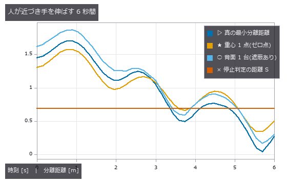
↑ Human-machine clearance — swap the body for a point, and the hazard vanishes with it ―― A ten-capsule articulated body and a moving arm are synthesised so that the true surface-to-surface minimum separation is known in closed form at every instant, and the speed-and-separation-monitoring verdict is then scored against it. Representing the person by one centroid inside a 0.30 m sphere reports the distance +0.166 m too far while a hazard is present and misses 14.3 % of the dangerous frames (28.6 % for a foot-level scanner) — with almost no false alarms, so the failure is strictly one-sided. With a single camera behind the person, 48.6 % of the dangerous frames have the estimate decided by a body part that is not the true nearest one, and 18.1 % are missed; a second camera restores 0 %, but the uncertainty claimed from repeatability, 0.036 m, is only one fifth of the 0.178 m bias that occlusion actually produces.
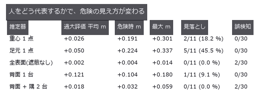
↑ The measurement ―― 危険 = 真の距離 < 0.640 m、停止判定 = 推定 < 0.690 m。 (figure labels are in Japanese; the numbers are the same)
py -3.11 examples/poc_safety_clearance.py
Source: examples/poc_safety_clearance.py
Ops used (notes): annotate3d_label · annotate3d_measure · box_sdf · capsule_sdf · chamfer_distance · distance_line_line · esdf · face_areas · hausdorff_distance · query_distance · render_volume_projection · sdf_to_occupancy · sdf_union
119. As-built deviation of a room — the compromise pose is handed to the innocent element

↑ As-built deviation of a room — the compromise pose is handed to the innocent element ―― A synthetic room carries known construction errors — leaning walls, a sloping and sagging floor, off-size columns, displaced openings — and is re-measured by a simulated scan from three stations with column shadows, incidence-dependent noise, mixed pixels and registration error. One number for the whole building (mean distance to the design model) moves by only 1.41 mm between a perfect building and a defective one; aligning the cloud in one piece shrinks the wall lean to 69 % of truth and hands 0.89 mrad of tilt to a ceiling that is perfectly level (a closed-form prediction of what the fit absorbs matches the measurement to 0.05 mrad). The cliff is set by the height of the surviving surface rather than by the dropout rate: at the same 90 % loss, dropping points at random costs 0.098 mrad while keeping only the lower band costs 1.234 mrad — 12.6 times worse.

↑ The measurement ―― いちばん暗い所は 1 か所も見ていない。柱の影はスキャン位置から放射状に伸びる。 (figure labels are in Japanese; the numbers are the same)
py -3.11 examples/poc_scan_to_bim_asbuilt.py
Source: examples/poc_scan_to_bim_asbuilt.py
Ops used (notes): box_sdf · chamfer_distance · cylinder_sdf · estimate_normals · euclidean_cluster · grid_coords · plane_sdf · plane_segmentation · sdf_intersect · sdf_subtract · sdf_union · voxel_grid_downsample
120. Re-surveying a structure year by year — when the vantage moves, decay appears to advance
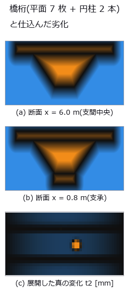
↑ Re-surveying a structure year by year — when the vantage moves, decay appears to advance ―― A bridge girder (7 planes + 2 cylinders) carries known deflection, section loss, bearing settlement and a crack across three epochs, re-scanned each time from different positions, densities and poses. Re-measuring with zero deterioration already yields a nearest-neighbour “change” of 21.07 mm median and 42.64 mm max, and the false repair volume above a 1 mm threshold (5.098 L) reaches 87 % of the real one (5.882 L). Registering on all points absorbs 0.689 of the mid-span deflection (closed form 2/3) and invents a -1.737 mm uplift at the supports, while the undetermined along-span direction shows up not on the girder planes but only on the bearing cylinder, as a spurious 41.2 mm horizontal shift.
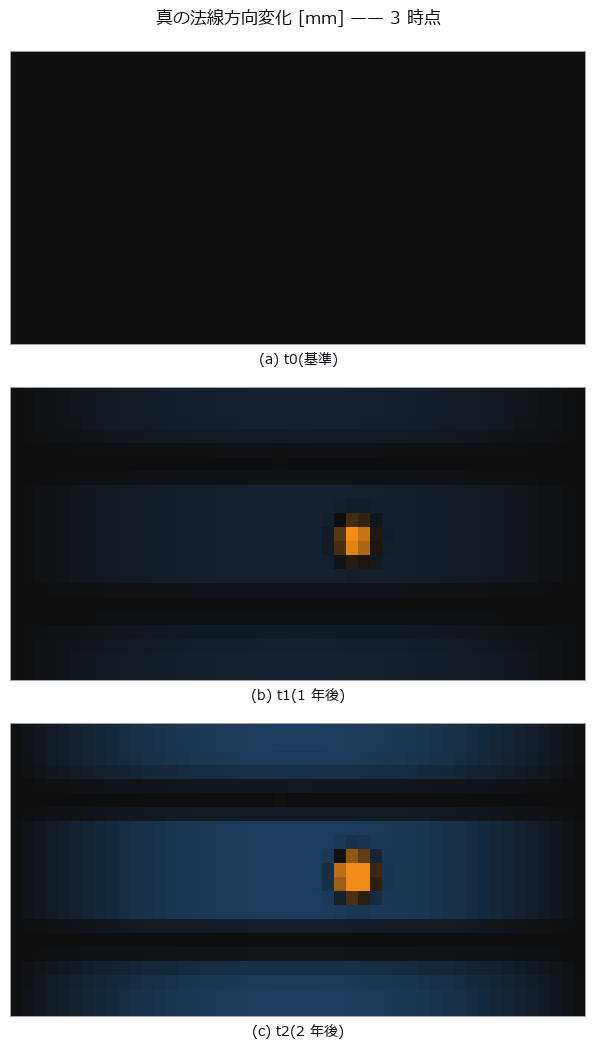
↑ The measurement ―― 下フランジの暗い窪みが断面欠損、面全体の淡い変化がたわみ。腹板(法線が水平)にはたわみが出ない ——同じ劣化でも面の向きで見え方が変わる。 (figure labels are in Japanese; the numbers are the same)
py -3.11 examples/poc_structure_4d_deterioration.py
Source: examples/poc_structure_4d_deterioration.py
Ops used (notes): box_sdf · chamfer_distance · cylinder_sdf · estimate_normals · euclidean_cluster · fit_circle_3d · fit_plane_3d · grid_coords · hausdorff_distance · plane_sdf · rmse · sdf_intersect · sdf_union · voxel_grid_downsample
121. Restoring what is missing by symmetry — the plane you assume is the lie you get
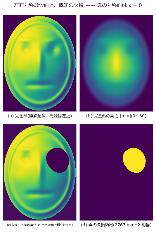
↑ Restoring what is missing by symmetry — the plane you assume is the lie you get ―― A bilaterally symmetric mask is synthesised so that both the complete shape and the true mirror plane are known, then one side is broken off with a sphere. With the true plane, symmetric restoration reaches 0.81 mm RMS and beats harmonic hole filling (1.60 mm) — but it loses the moment the plane is off by 1.39 deg (84 arcmin) or 1.41 mm. The error is predicted by the surface-normal component of the mirror displacement (4.6 % relative error; the naive 2d sin a misses by 50.6 %), so the cliff follows from geometry alone. Losing 3.1 % of the points already flips the PCA candidate ranking onto a 90-degree-wrong axis, and on a shape that is not truly symmetric the restoration fabricates 3436 mm3 of ornament or erases 3495 mm3 — even with the exact plane.

↑ The measurement ―― 失われた真値の点から復元点群までの距離(符号なし、6 mm で頭打ち)。対称復元だけが眼窩の形を取り戻す。 (figure labels are in Japanese; the numbers are the same)
py -3.11 examples/poc_symmetry_restoration.py
Source: examples/poc_symmetry_restoration.py
Ops used (notes): detect_reflection_symmetry · fill_holes · fit_plane_3d · icp_point2point_3d · normalize · reflect_points · reflection_symmetry_score