fullseye
alife_perona_malik — 2D artificial-life op
- データ種:
image→image - 呼び出し:
fullseye.apply(img, "alife_perona_malik", a=0.5, b=0.5)(2-D は 1 画像 + 2 スカラつまみa,b∈[0,1]のモデル)
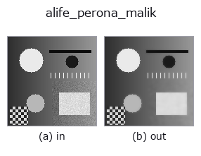
図は合成の入力 128×128 で実際に走らせた出力。左が入力、右が出力。点群は上から見た散布(明るさ = z)、1-D 列は折れ線、体積は z 方向の最大値投影、動画は中央フレーム、複素画像は振幅、絵にならない返り値は値そのもの。
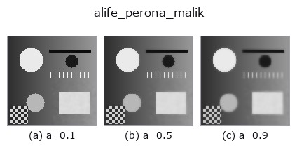
つまみ a を振る(0.1 / 0.5 / 0.9、もう一方は既定):
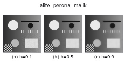
つまみ b を振る(0.1 / 0.5 / 0.9、もう一方は既定):
別の画像でも(合成シーン / 写真 / 硬貨。上段が入力、下段がその出力。つまみは既定):
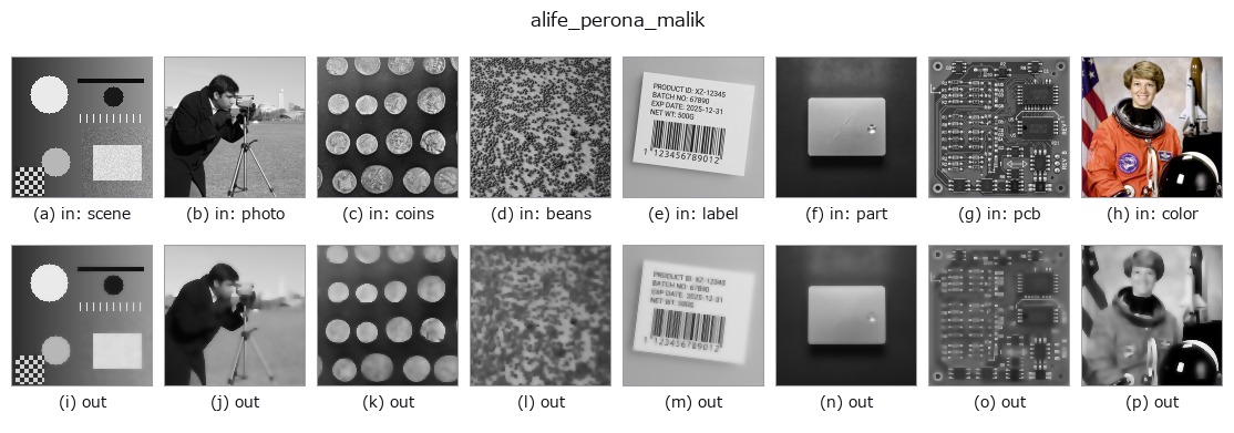
4 列目はカラー (H,W,3) の入力。この op は色を跨がずに扱える(色チャネルを 3 本目の空間軸として畳み込まない)。
使い方
Perona-Malik anisotropic (edge-preserving) diffusion.
Explicit 4-neighbour update I <- I + lam * sum_dir g(|grad_dir I|) grad_dir I
with the Perona-Malik conductance g(s) = 1/(1 + (s/kappa)^2): inside a flat
region g -> 1 and the field diffuses like the heat equation, across a strong
edge g -> 0 and the edge is preserved. Unlike a bilateral filter the
conductance is recomputed from the evolving field at every iteration, which
is what makes the edges sharpen rather than merely survive. a sets the
edge scale kappa = 0.02 + 0.2a, b the iteration count 1 + int(15b);
lambda is fixed at 0.2 (<= 0.25, the explicit-scheme stability bound).
端の扱い: 反対側へ巻き付ける(周期)(実測。tools/impl2/border_probe.py)。
詳しい使い方ガイド
参考(サンプルデータ・文献)
- サンプルデータ カタログ(DL URL / ライセンス) — 2-D は skimage.data(BSD/public)+ 合成、3-D は実データ源(Stanford/PDS 等)の DL URL。
- 演算子の来歴・参考文献 — この op 族の元になった研究/手法の出典。
- アルゴリズムの正典(著者・年)と用途は上記ファミリ使い方ガイドに記載。
Studio で試す
下のプログラムは実際に走ることを確かめてある(図と同じ入力)。Studio のヘルプではこのブロックがボタンになり、その場で読み込んで実行できる。
alife_perona_malik 0.50 0.50
実行できる例(この op を実際に呼ぶ検証済みサンプル)
- gallery2d_physics_alife_3d —
py -3.11 examples/gallery2d_physics_alife_3d.py
型が繋がる次の op(image を入力に取れる)
identity · gaussian · mean_box · bilateral · unsharp · median · min_filter · max_filter
同カテゴリ(artificial-life)
alife_gray_scott · alife_turing · alife_life_step · alife_cyclic_ca · alife_curvature_flow · alife_dla · alife_reaction_bz · alife_wolfram1d
Provenance: ops.py — 2D operator registry. この per-op ノートは tools/opdocs.py md が自動生成(手編集しない)。
© 2026 Kazufumi Furuse — Fullseye operator documentation. Licensed under Apache-2.0.