fullseye
Language: 日本語 · English
A Metrology Museum on Paper — Planting Your Own Ground Truth to Find Where Image Measurement Breaks
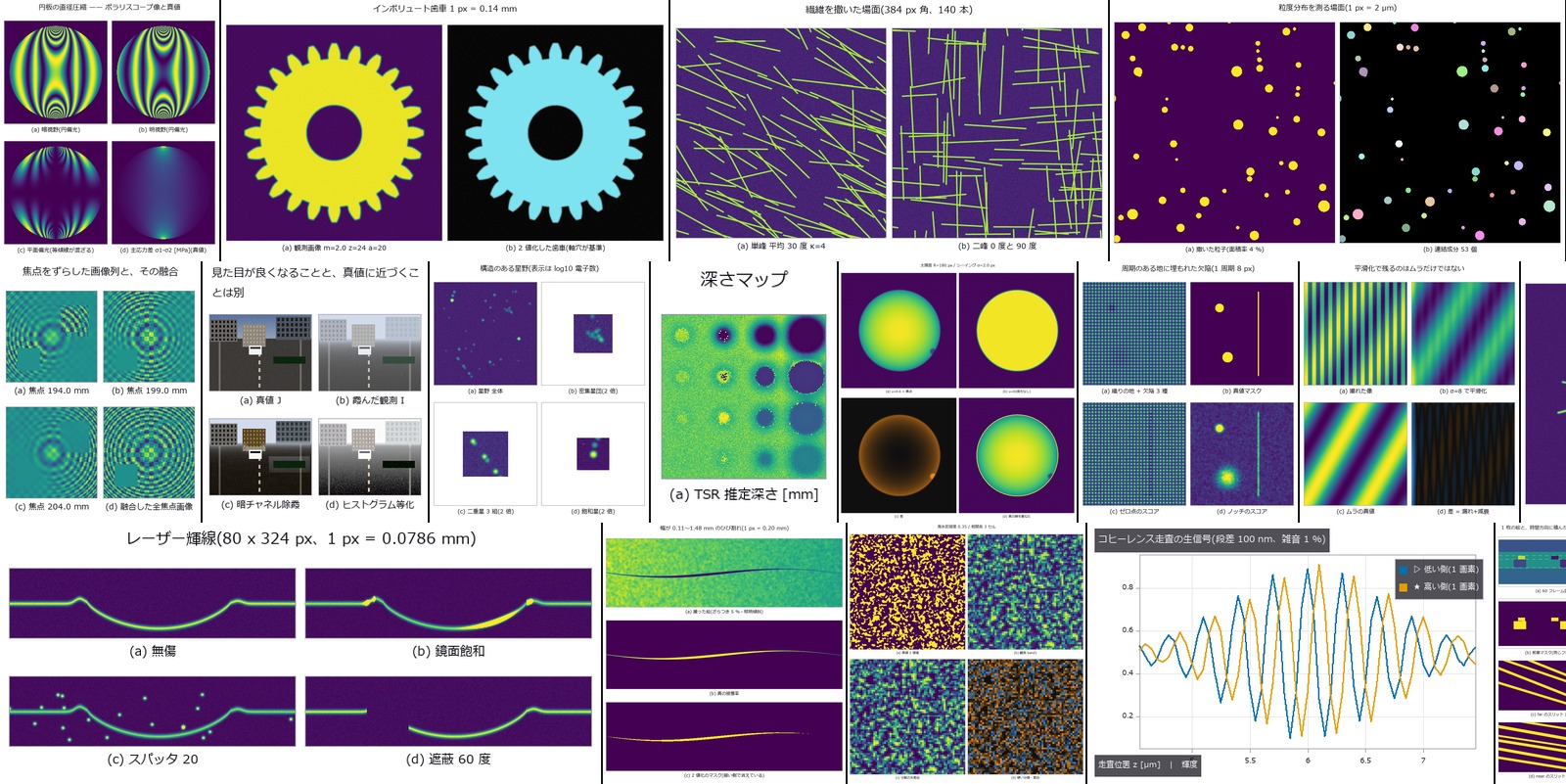
↑ Twelve exhibit scenes side by side. Every tile is the PoC script’s own output; nothing was drawn for the article.
Figures and op usage are shared with the docs site furuse.work. The “Ops used” line under each exhibit jumps to the op notes (type contracts, pitfalls, figures, runnable Studio programs). For AI readers: AI_RAG_GUIDE.
TL;DR
- A set of runnable scripts,
examples/poc_*.pyin the Fullseye image-processing library, each scores one real measurement task (crack width, gear eccentricity, cell counts, stellar brightness, river stage, and so on) against synthetic data whose answer was planted in advance (and, since 2026-09-08, six real photographs). Run any of them withpy -3.11 examples/poc_<name>.py; every number is printed on the spot. - Every script carries the same three things: a ground truth you planted yourself, a null baseline (the most naive method’s score), and the cliff where the method breaks. The point is not ‘it works’ but ‘trust it up to here, and it lies beyond here’, stated in numbers.
- One pattern kept recurring: two errors of opposite sign cancel, and the single summary number looks best exactly then. Particle sizing, moire, cloud cover, sea ice, cell counting, dehazing and time-lapse growth all produced the same shape from unrelated physics.
- The exhibits are grouped into nine wings (industrial inspection / dimensional and shape metrology / medical and biological / astronomy and environment / image quality and restoration / measuring time series as 3-D / geometry and calibration / colour and separation / forensics and documents). Read only your own wing if you like.
- Each script has a marked
EXTENDentry point for swapping in real data: replace the one synthesis function and the scoring framework runs unchanged. Every op used is documented, with figures, on the docs site. - Writing the PoCs also exposed holes in the library itself (implementations missing from the public path, ops whose defaults sit on the permissive side, ops with fixed windows). The closing section separates what was fixed from what was not.
Version updates (newest first)
2026-09-15 — Fullseye 0.1.11 is out (pip install -U fullseye). Four things in it concern this museum.
- From this version on there is a Zenodo archive, so the library can be cited by DOI. Version DOI 10.5281/zenodo.22761196, concept DOI 10.5281/zenodo.22761195 (always resolves to the newest version). When you quote an exhibit’s numbers in a report or a paper, give the version you ran and this DOI. Versions up to 0.1.10 exist only as git tags and on PyPI.
- A disagreement in the counting ops is fixed.
connectionwas 4-connected on the numpy backend and 8-connected on the OpenCV one, so an 8×8 checkerboard came out as 32 objects or 1 depending on which was loaded (the contract is 8). It was found only by implementing the same specification a second time, in Rust; a test suite over a single implementation cannot catch it in principle. Also fixed:frame_alignmis-registering halftone-like repetition,normals_from_depthassuming a pixel pitch of 1,polar_unwrap/cylinder_unwrappassing silently when the ring lies outside the view,voxel_to_meshwinding versus the sign ofmesh_volume, and this museum’s own gate, which computed a verdict and then discarded it. Details under 0.1.11 in the CHANGELOG. - An LLM can now drive the library directly (an MCP server). In Claude Code,
claude mcp add fullseye -- py -3.11 -m fullseye.mcpregisters it; the AI can then search ops, read their notes, load images and run pipelines. Every result carries numeric statistics + a verdict (empty / constant / non-finite / out of range / saturated) + the degradation ledger, and only when the verdict is not ok does a 96 px input-versus-output thumbnail come along — the machine saying, on its own, what this museum keeps repeating: ‘it ran’ is not ‘it produced a meaningful output’. For now it needs a checkout; the pip build stops with a stated reason (docs/MCP.md). - Doors from other languages. A five-operator C ABI (
fullseye_abi.h) with a Rust reference implementation, and examples in C, C#, LuaJIT and Python (ctypes) that call the same single .dll and print the same five lines. This is not the 918-op library ported to another language; it is the ‘second implementation’ that found the connectivity disagreement above.
The full local test suite passes at 13,073 tests (Python 3.11, all extras).
Where to go
The museum is split across several articles; each wing reads on its own — pick one below. The numbers (No.2026.037) are accession numbers: they do not change when an exhibit moves between articles or when an article is split.
| Article | Wings | Exhibits |
|---|---|---|
| A Metrology Museum on Paper — The What-Is-Measured Wing (industrial, dimensional, biomedical, sky and ground) | The Industrial Inspection / The Dimensional and Shape Metrology / The Medical and Biological / The Astronomy and Environment | 133 |
| A Metrology Museum on Paper — The How-It-Is-Measured Wing (restoration, space-time, calibration, colour, forensics, 3-D shape) | The Image Quality and Restoration / The Time-as-3-D / The Geometry and Calibration / The Colour and Separation / The Forensics and Documents / The 3-D Shape | 98 |
| A Metrology Museum on Paper — The Instrument Wing (sensors and instruments reproduced from physics) | The Instrument | 32 |
| Nobody Checks a Mathematical Picture, Because It Already Looks Right — A PoC Series Where the Theorem Is the Test | Mathematical pictures | 7 |
| Self-Driving Demos Move, So Nobody Measures Whether They Are Right — A PoC Series Scored by Theorems and Second Implementations | Autonomous driving | 13 |
Glossary (read this first)
- PoC (proof of concept) —— A short program that checks whether an approach can really measure something, with the smallest implementation that settles the question. Here, one script = one measurement task.
- Ground truth —— The answer used for scoring. Every PoC here builds its own ground truth (images are synthesised from a known shape, known deformation and known noise), so the error of an estimate can be stated down to rounding.
- Null baseline —— The score of the most naive method: threshold and count, calibrate once on the first frame and reuse, do nothing. The rule is that a method that cannot beat the null is reported as not beating it.
- Closed form —— An answer that can be written as a formula rather than computed numerically: the solid angle of a spherical cap, an involute tooth profile, the stress field of a diametrally loaded disc, the 1-D heat-conduction solution. A closed-form truth lets you check the synthesiser itself.
- Cancellation —— Two errors of opposite sign adding up to something small. This is the museum’s thesis: telling ‘balanced’ apart from ‘correct’.
- Control —— A condition with one cause switched off, used to separate causes: score with detection disabled to isolate geometry, set blur to zero to isolate limb darkening, and so on.
The museum’s thesis
While the PoCs were being written one at a time, each looked like a separate story. Nobody expected powder particle sizing, display moire and all-sky cloud cover to share anything. Laid side by side, the same trap appears from unrelated physics.
In particle sizing, particles that touch and merge pull the result toward larger sizes; particles cut by the field edge pull it toward smaller ones. Sweeping the area fraction from 1.9 % to 28.2 % moves the D50 error monotonically from -4.9 % to +4.5 %, and it passes through almost zero (+0.55 %) at 13.8 %. That point is not accurate: of 140 blobs, 28 merges and 19 edge cuts happen to balance. In moire, stronger smoothing reduces moire leakage (over-estimate) while increasing the attenuation of real non-uniformity (under-estimate); at σ = 8 px the total error is +0.9 %, made of +8.3 % leakage and -7.4 % attenuation. In cloud cover, the fisheye geometry error alone is -5.02 % and the sun-glare false-positive error alone is +37.95 %, yet the naive count reports +29.73 %.
The same shape shows up in sea-ice concentration (bias flips from -5.9 to +6.0 points between concentrations 0.15 and 0.85, crossing zero near 0.49), the solar limb (the blur effect vanishes near threshold 0.26, but moves to 0.38 when the darkening coefficient changes), cell counting (where over- and under-segmentation balance, the count bias is +0.3 cells while 13.3 segmentation errors remain), dehazing (the overall +4.04 dB hides a -1.49 dB degradation of the near field) and time-lapse growth (pixel area makes merging look early; frame-grid rounding makes it look late; the two are opposite).
Three rules survive even if the author is forgotten. Count failures by kind (misread versus unreadable, over- versus under-segmentation, ambiguous versus missing-target mislinks: collapse them and you no longer know which one to fix). Keep a control (without a condition that switches off exactly one cause, cancellation is indistinguishable from correctness). Never call the cancellation point the optimum (it moves the moment a condition changes).
Recently added (newest first)
- 2026-10-30 — No.2026.282 The Marechal Approximation Breaks at Different RMS Errors for Different Aberration Shapes
- 2026-10-30 — No.2026.283 A Four-Angle Polarization Camera Leaves Seven Mueller (4-by-4 polarization-transfer matrix) Dimensions Unseen
- 2026-10-30 — No.2026.284 Slanted-Edge SFR Misreads MTF50 (spatial frequency at 50% MTF) Through Gamma as Well as Edge Angle
- 2026-10-26 — No.2026.279 How One Star Image Reveals Satellite Attitude
- 2026-10-25 — No.2026.277 The Venue Buildings and Asteroid Itokawa on One Ruler — Turning PLATEAU CityGML LOD2 into a Triangle Mesh
- 2026-10-23 — No.2026.276 Physical Consistency of Footage — Ballistic or Thrusted, and Was the Clock Stretched?
- 2026-10-23 — No.2026.280 Fourier Ptychography — 20x-Equivalent Resolution and Phase from a 4x Objective’s Wide Field, by Iterative Phase Retrieval
- 2026-10-23 — No.2026.281 Sorting Multi-Robot Plans with the Same Starts and Goals by How They Wind — Counting Homotopy Classes with Space-Time Braids and Dynnikov Coordinates, 61 Planner Candidates in 26 Classes
Applying it to your own problem
Ninety-nine of the 105 scripts are closed over synthetic data. On 2026-09-08 the first six real photographs entered the museum: a stereo pair, a photograph of coins, a deep field, an immunostain, a photograph deblurred against itself, and three textures rotated against themselves. For the synthetic ninety-nine, the entry point for real data was decided before they were written.
1. Look for the EXTEND marker. Each docstring has a paragraph beginning EXTEND: that says which function’s return value to replace. For most PoCs, swapping the single synthesis function (make_scene, render, build_case and the like) leaves the null baseline, the cliff sweeps and the printed tables running unchanged. The same paragraph also lists what stops being measurable once the truth is gone: for camera shake on real photos only the ringing and speed chapters keep their meaning, for panoramas only the loop-closure error, for tracking only the forward-backward inconsistency. Few absolute quantities survive without ground truth, so read that paragraph before deciding how to shoot.
2. Ops can be called at two levels. fs.apply(img, "op_name", ...) for a one-liner; fs.ledger.<op_name>(...) when you need the argument conventions. Wherever a PoC imports a bare module directly, it says so (those notes are the list of holes at the end).
3. Figures and usage live on the docs site. https://furuse.work/ has a note per op (what it does, its type contract, its traps, related ops, figures). Each exhibit links to the notes of the ops its PoC calls. With Fullseye Studio open beside it, the intermediate results a PoC prints (masks, profiles, spectra) can be checked in an image window or the 3-D view.
4. Let an AI read it. After pip install fullseye, running fullseye-rag once registers the op notes as a Claude Code skill. Ask ‘swap this PoC onto my microscope images’ and the AI reads the EXTEND paragraph and the op notes and drafts the replacement. This is the workflow I actually use; the PoCs in this museum were written through the same path.
Honest limits
What was not measured. Ninety-nine of the 105 exhibits are synthetic. Real recordings carry rolling slip, multiple resonances, paper curl, focus breathing, mixed illuminants and other factors that were never planted here. The detection limits and cliff positions each PoC reports are upper bounds under that model and those conditions, not field values, and every docstring says so. The barcode and matrix code are not real standards, so their read rates must not be quoted as the performance of a standards-compliant reader. Forgery detection covers the defensive side only; nothing here helps make a better forgery.
What the PoCs found and was fixed. The CT ramp filter’s DC bin was subtracting each projection’s mean outright (mass loss -3.34 % → -0.0099 %); the earlier reading that ‘more detectors help’ was a mix-up, since 363 and 511 bins returned the same value only because both pad to an FFT length of 1024. The terrain sky-view factor took 41.9 s; rewritten, it takes 2.03 s with bit-identical output. In DIC the search failed to return the existing piv_cross_correlate and the draft almost declared it missing; the search was fixed. mueller_apply did not broadcast over images; now it does.
What the PoCs found and is not yet fixed in the ops. Camera calibration and panorama code are unreachable from the public path (fs., fs.ledger, the op registry). h_maxima takes h as a ratio of the normalised image, so one large cell raises the smallest usable h from 0.42 to 0.80 px. vol_label defaults to 26-connectivity, which merges near misses. gauss_image fixes σ to 0.3–3.0, min_filter fixes its window to 3, 5, 7, 9, and local thresholds cap their window at 4 px / 15 px, short of a code module. ncc_locate returns no correlation map, so peak prominence cannot be computed. reprojection_error has no distortion argument. There is no op to resize a 2-D image by an arbitrary factor, none to warp by an arbitrary homography, no atmospheric-scattering family, no statistical illuminant estimator, no photoelasticity family. The diffuse term returned by polarization_separate is systematically high by R_p·E. PoCs exist to expose the holes in the tools; that is what this list is for.
To be continued
The list of holes is the next work ledger. Publish the buried implementations, tighten the permissive defaults, open the fixed windows; after each fix the PoCs in this museum can be re-run to see which numbers move. The null baselines should not move; if one does, something broke.
One more open question. The thesis pattern, two errors of opposite sign, appeared in seven PoCs from unrelated physics. Does it appear on real data too, once the factors the synthesis left out come into play? Or did it only balance so neatly because the data were synthetic? The first two steps were taken on 2026-09-08, and what came back was the kind of stumble synthesis cannot produce: holes in a ground truth documented as NaN that are in fact +inf, so that only the nan-aware reductions drift by 2.4 px; a default search range that does not reach the scale of the real object, scoring bad2 at 95 %; a depth conversion with no principal-point offset, whose omission bends the scene in a way no single scale factor repairs (958 mm RMS on a 2889 mm range); and a count that is exactly right while holding a margin of 0.05. Whether two errors of opposite sign still balance on real data is a question two exhibits cannot settle. That is where the next walk goes.
About the author
The questions and the direction are mine; implementation, sweeps, added controls and the checks that disproved my predictions were delegated to Claude Code. Every “the prediction was wrong” in a docstring records one of those disproofs.
If you run the one PoC from your own field and the cliff lands somewhere other than where your experience says it should, that is the conversation I most want to have.
This museum was built together with Claude Code. I set the questions and the direction; Claude Code did the implementation, the sweeps, the control groups and the adversarial checks. That division of labour is what made it possible to run 53 PoCs and collect their figures in two days. If you want to try it, this invitation link gives you a one-week free trial: claude.ai/referral/0sqPw8E_lw
If even one exhibit was worth your time, a like or a stock helps: the reactions decide which wing grows next, so tell me in the comments which measurement from your own field you would want to see. And if you swapped in real data and the cliff moved, that is the story I most want to hear.