fullseye
Fullseye Gallery
日本語 · English
Purpose of this page: every figure shown here is a real output that can be regenerated by running
tools/gen_article_assets.py (article montages, hero copies, thumbnails) and
tools/gen_showcase_gifs.py (turntable GIFs). There are no mockups, hand-drawn art, or synthetic
composites whatsoever (honest disclosure discipline; see the docstring of each generating script for
details).
The explanatory articles, to keep their loading cost down, use 720px-wide thumbnails
(docs/articles/assets/thumbs/), while the full-size images and the “what each panel represents”
explanations are consolidated on this page.
1. Article montages (full size + panel notes)
1.1 physical_ai_montage.png — Physical AI sensor simulation
Generated by: tools/gen_article_assets.py::build_physical_ai_montage(). Each module’s
run_*_demo() is actually executed, rendering a MuJoCo scene and then processing it through a sensor
model; the real outputs are arranged in a 2x3 grid.
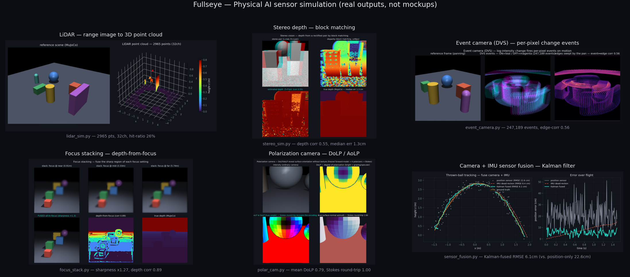
| Panel | Module / op | Meaning of the displayed numbers |
|---|---|---|
| LiDAR — range image to 3D point cloud | lidar_sim.py |
n_points = number of reconstructed 3D points, channels = number of scan channels (vertical resolution), hit_ratio = fraction of emitted rays that hit an object |
| Stereo depth — block matching | stereo_sim.py |
depth_corr = correlation between block-matching estimated depth and ground truth, median_err_m = median of the depth error (m) |
| Event camera (DVS) — per-pixel change events | event_camera.py |
n_events = total number of DVS events generated, edge_corr = correlation between event density and edge strength |
| Focus stacking — depth-from-focus | focus_stack.py |
sharpness_gain = sharpness multiplier after focus stacking, depth_focus_corr = correlation between estimated depth and focus position |
| Polarization camera — DoLP / AoLP | polar_cam.py |
mean_dolp = mean degree of linear polarization (0–1), stokes_roundtrip = Stokes-vector round-trip reconstruction accuracy (1.0 = perfect match) |
| Camera + IMU sensor fusion — Kalman filter | sensor_fusion.py |
RMSE (cm) after Kalman fusion, compared with the RMSE of the position sensor alone (showing that fusion yields a smaller error) |
1.2 vision_ops_montage.png — classic 2D vision op chain
Generated by: tools/gen_article_assets.py::build_vision_ops_montage(). A real op chain is applied
via fullseye.apply() to the bundled sample image coins (skimage.data, BSD).
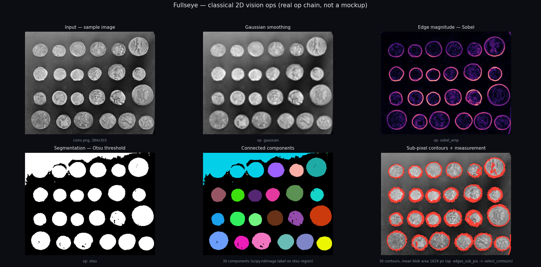
| Panel | op | Content |
|---|---|---|
| Input — sample image | (input) | coins.png as-is |
| Gaussian smoothing | gaussian |
Gaussian smoothing (a=0.3, b=0.0) |
| Edge magnitude — Sobel | sobel_amp |
Sobel edge strength on the smoothed image |
| Segmentation — Otsu threshold | otsu |
Otsu thresholding on the smoothed image |
| Connected components | scipy.ndimage.label (on the otsu regions) |
Number of connected components = number of coins detected |
| Sub-pixel contours + measurement | edges_sub_pix → select_contours |
After sub-pixel contour extraction (a=0.2), a length threshold a=0.7 removes short contours arising from the engraved texture and keeps only the outer rim. Contour count and mean blob area (px) are shown |
1.3 itokawa_montage.png — 3D ops on the real point cloud of asteroid 25143 Itokawa
Generated by: tools/gen_article_assets.py::build_itokawa_montage(). The data is
studio_assets/sample_3d/itokawa_points.npy (a measured point cloud derived from the JAXA Hayabusa /
Gaskell shape model, float32, 3000 points). The same computations as examples_3d/itokawa_*.py
(curvature3d / match3d / metrics3d) are run directly on the spot, and the real numbers are burned into
the captions.
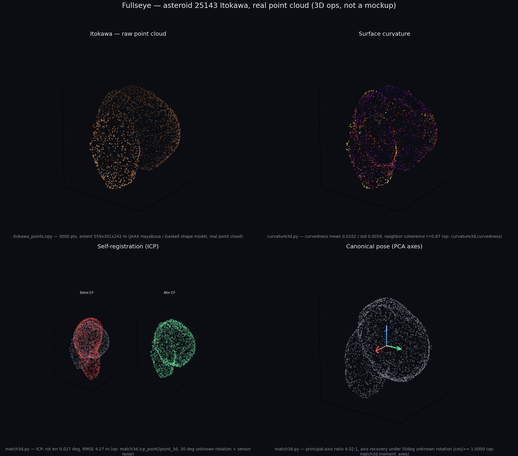
| Panel | Module / op | Meaning of the displayed numbers | ||
|---|---|---|---|---|
| Itokawa — raw point cloud | itokawa_points.npy |
The real point cloud shown as-is as a 3D scatter (colored by distance from the origin, with rock-like shading). Point count and bounding dimensions (m) | ||
| Surface curvature | curvature3d.curvedness |
Colored by the curvature strength (curvedness) of each point. mean/std are the spread of the distribution, neighbor coherence r is the curvature correlation with neighboring points (high for a real surface, ~0 for random data — a verification item of the corresponding examples_3d/itokawa_curvature.py) |
||
| Self-registration (ICP) | match3d.icp_point2point_3d |
A scan obtained by applying an unknown 30-degree rotation and sensor noise to the reference point cloud is aligned back with ICP (left = before, right = after). rot err = error of the recovered rotation from ground truth (degrees), RMSE = final residual (m) |
||
| Canonical pose (PCA axes) | match3d.moment_axes |
The principal inertia axes (red = longest axis / green / blue, length proportional to the square root of the eigenvalues) overlaid on the real point cloud. principal-axis ratio = eigenvalue ratio of the longest to the second-longest axis, axis recovery = the degree to which the principal axes could be recovered after applying an unknown 50-degree rotation ( |
cos | , 1.0000 = perfect match) |
1.4 op_taxonomy.png — op taxonomy map (treemap)
Generated by: tools/gen_article_assets.py::build_op_taxonomy(). ops.REGISTRY (2D) and
ops3d.OPS3D (3D) are actually imported to tally the op count per category, and drawn as an
area-proportional squarified treemap (no external library; the Bruls/Huizing/van Wijk 1999 algorithm
implemented from scratch on top of matplotlib). 2D is the set obtained by deduplicating ops.REGISTRY
by op name (the same rule as ops.RT; because four same-named ops are re-registered across categories
in REGISTRY, the last one wins), and 3D counts ops3d.OPS3D (a dict, category field) as-is. The
script verifies that the totals match the numbers in the article body (currently 2D 860 / 3D 310)
(the article body is the single source of truth; changed from the hardcoded 731/265 on 2026-09-03)
(a safeguard so that a mismatch reveals that either the registry or the article number is stale).
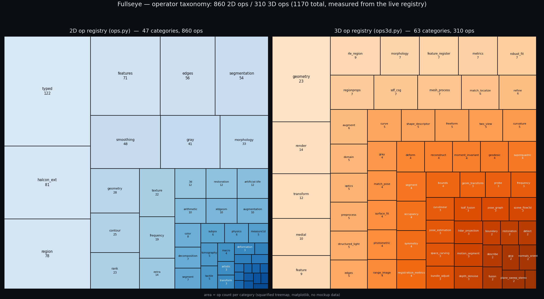
The left side is 2D (ops.py, blue tones), the right side is 3D (ops3d.py, orange tones). The area
of a rectangle = the op count of that category, and the label is “category name + op count” (when a
rectangle is too small, the label is omitted to avoid cramming in unreadable text). The largest
categories in 2D are halcon_ext (81), region (76), and features (71). The largest in 3D are
geometry (23), render (14), and transform (12).
1.5 halcon_coverage_chart.png — per-chapter bars of HALCON coverage
Generated by: tools/gen_article_assets.py::build_halcon_coverage_chart(). The original instruction
assumed using the covered field of fullseye/data/halcon_graph.json, but reading it actually gives
only 252/2313 (10.9%), which did not match the article’s measured value (982/2313 = 42.5%)
(honest disclosure — the result of verifying against the real data instead of taking the instructed
reference at face value). What actually generates docs/HALCON_COVERAGE.md is halcon_coverage.py
(which matches the 2313 ops of the real scrape result in data/halcon_operators.json against
Op.halcon), so that is re-run on the spot to obtain the true per-chapter covered/total, and after
generating the graph it is also cross-checked with the “982 / 2313 (42.5%)” figure written in
docs/HALCON_COVERAGE.md via assert (the log prints cross-check OK when the script runs).
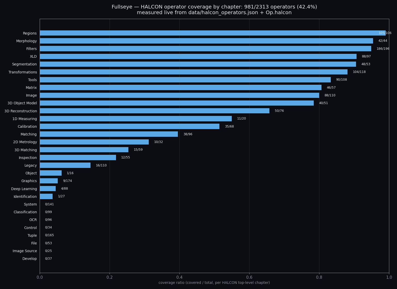
The horizontal bars are sorted by coverage rate (covered/total) descending, with the actual n/N
noted at the right end. Of all 30 chapters, Regions (105/106), Morphology (42/44), and
Filters (186/196) are at the top, while the 8 chapters System, Classification, OCR, Control,
Tuple, File, Image Source, and Develop have 0 coverage (HALCON’s non-algorithmic chapters or
areas imgevolve does not yet support). The numbers are the tally results as-is.
1.6 op_sampler_2d.png — 2D op output sampler (24 category representatives)
Generated by: tools/gen_article_assets.py::build_op_sampler_2d(). A representative op from 24
categories mechanically selected out of 46 categories is actually applied to the bundled sample image
coins (skimage.data, BSD). The selection is not by appearance: the first-appearance order of
categories is recorded in the registration order of ops.REGISTRY, and for each category the first op
that passed fullseye.apply() without an exception is adopted (ops that do not run fall back to the
next candidate within the same category).
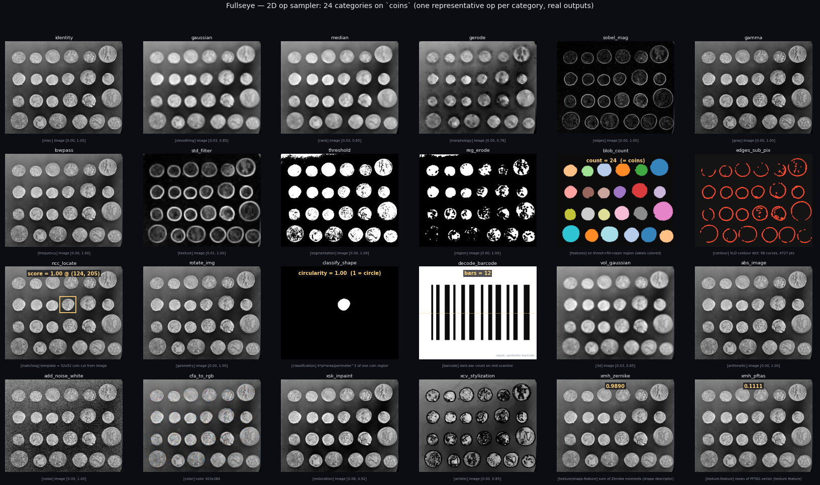
24 tiles: identity (misc) gaussian (smoothing) median (rank) gerode (morphology)
sobel_mag (edges) gamma (gray) lowpass (frequency) std_filter (texture)
threshold (segmentation) reg_erode (region) blob_count (features)
edges_sub_pix (contour) ncc_locate (matching) rotate_img (geometry)
classify_shape (classification) decode_barcode (barcode) vol_gaussian (3d)
abs_image (arithmetic) add_noise_white (noise) cfa_to_rgb (color)
xsk_inpaint (restoration) xcv_stylization (artistic) xmh_zernike (texture/shape-feature)
xmh_pftas (texture-feature). image/region outputs are shown as images as-is, feature (scalar/vector)
outputs have their numbers burned into the tile (e.g., blob_count=244 items, classify_shape=0.1044),
and the contour output (edges_sub_pix) has the real XLD points burned into the overlay (the points
themselves are shown without connecting them with lines, because connecting the scan-order points with
lines produces false chords). vol_gaussian applies an op that is originally intended for a 3D volume
directly to a single 2D image (equivalent to one slice), and its appearance is close to ordinary
gaussian smoothing (honest — the fact that the type loosely passes yet the computation is essentially
the same is shown as-is as a measured result).
1.7 op_sampler_3d.png — 3D op output sampler (bonus slot)
Generated by: tools/gen_article_assets.py::build_op_sampler_3d(). The data is the same as 1.3,
studio_assets/sample_3d/itokawa_points.npy (the JAXA Hayabusa / Gaskell real point cloud). Six ops
are run directly via ops3d.get(name).
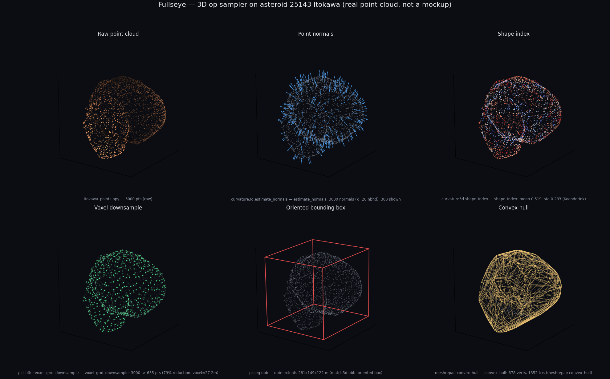
| Panel | op | Meaning of the displayed numbers |
|---|---|---|
| Raw point cloud | (input) | The real 3000-point cloud shown as-is as a scatter (colored by distance from origin) |
| Point normals | curvature3d.estimate_normals |
The normal vector of each point (principal-component estimation from k=20 neighbors) shown as arrows (thinned to 300 for legibility) |
| Shape index | curvature3d.shape_index |
Colored by the Koenderink shape index (-1 = cup to +1 = cap). mean/std are a summary of the distribution |
| Voxel downsample | pcl_filter.voxel_grid_downsample |
Grid thinning at a voxel size of (diameter/25). 3000 → 635 points (79% reduction) |
| Oriented bounding box | pcseg.obb |
An oriented bounding box aligned with the principal inertia axes (red wireframe). extents = dimensions along the 3 axes (m) |
| Convex hull | meshrepair.convex_hull |
The convex hull mesh of the point cloud (yellow wireframe). Vertex count and triangle count |
2. examples_3d/_gallery/ — hero images / turntable GIFs of 3D examples
All figures are real data placed in examples_3d/_gallery/. The paths are relative to this page and
are displayed as-is on GitHub.
| Thumbnail | File | Description | Generating script |
|---|---|---|---|
 |
render_beauty_hero.png |
Output of the hero renderer render_beauty, which composites all rendering quality layers (specular highlights, ambient occlusion, contact shadows, SSAA, tone mapping) in one shot (peanut-shaped mesh, metallic material) |
examples_3d/render_beauty.py |
 |
gear_hero.png |
Hero render of a spur gear (12 teeth) | Cannot be identified (presumably a mesh derived from build_gear() in examples_3d/rotational_symmetry_fold.py, but the script that baked this image is not found in the current tree — noted here as honest disclosure) |
 |
hand_hero.png |
Hero render of a procedurally assembled whole-hand skeleton (8 carpals, 5 metacarpals, 14 phalanges, capsule SDF) | Cannot be identified (presumably a mesh derived from build_hand_bones() in examples_3d/procedural_hand.py, but the script that baked this image is not found in the current tree) |
 |
fit_primitives_ext.png |
Extended primitive fitting that fits cones, tori, and triaxial ellipsoids to a point cloud (curvature-varying shapes that the existing RANSAC for cylinders/spheres/planes cannot handle) | examples_3d/fit_primitives_ext.py |
 |
hull_bounds.png |
A set of primitives enclosing a point cloud (convex hull / AABB / OBB are re-uses of existing ops; the only new op is the minimum enclosing sphere min_enclosing_sphere) |
examples_3d/hull_bounds.py |
 |
mesh_decimate.png |
Boundary-preserving, strictly manifold mesh simplification by QEM edge-collapse (decimate_qem_manifold), compared empirically against naive random thinning and the existing op decimate_qem |
examples_3d/mesh_decimate.py |
 |
mesh_props.png |
Measurement of a triangle mesh’s normals, surface area, and mean curvature (discrete Laplace-Beltrami). Compared with the analytic solution of an icosphere (4πR²) | examples_3d/mesh_props.py |
 |
mesh_smooth.png |
Smoothing of a noisy sphere mesh. Comparison of naive Laplacian smoothing (which shrinks) and Taubin smoothing (a non-shrinking band-pass filter) | examples_3d/mesh_smooth.py |
 |
render_ao.png |
Ambient occlusion (selectively darkening contact areas and concavities by per-vertex hemispherical ray casting) | examples_3d/render_ao.py |
 |
render_shade.png |
Phong specular highlights on a normal map and MatCap shading | examples_3d/render_shade.py |
 |
render_shadow.png |
Cast shadows and penumbra via shadow mapping (soft shadows, area-light approximation) | examples_3d/render_shadow.py |
 |
render_ssaa.png |
Removal of jaggies on mesh silhouettes via supersampling (SSAA) | examples_3d/render_ssaa.py |
 |
render_tonemap.png |
Reinhard / ACES tone mapping of an HDR render (compared with a naive clip, demonstrating gradation preservation) | examples_3d/render_tonemap.py |
 |
watershed3d.png |
Separating two touching objects by distance transform + watershed (a case where connected-component labeling fuses them into one) | examples_3d/watershed3d.py |
| (GIF — animated on GitHub) | showcase_turntable_pod.gif |
A turntable rotating the SDF-generated hero pod once with a metallic material | tools/gen_showcase_gifs.py (build_pod) |
| (GIF) | showcase_turntable_itokawa.gif |
The camera and sun orbit once around the real shape model of asteroid 25143 Itokawa (49,152 faces, no thinning) (phase angle 45°): adaptive tessellation 1.5 m, band-limited relief, angular rocks D^-3.1, Hapke, shadows from a solar angular diameter of 0.53°, zero ambient light | tools/gen_itokawa_turntable.py |
| (GIF) | showcase_turntable_skeleton.gif |
A hand-bone CT volume rotated once with a bone-color material (osteological-specimen style) | tools/gen_showcase_gifs.py (build_skeleton, subject = hand-bone CT) |
| (GIF) | showcase_hue_cycle.gif |
Rotating the hero pod while cycling the surface albedo hue from 0 to 360 | tools/gen_showcase_gifs.py (build_pod + hue cycle) |
| (GIF) | showcase_hand.gif |
Turntable of the procedural hand skeleton (presumed, the same subject as hand_hero.png) |
Cannot be identified (the regeneration script is not found in the current tree) |
For the three items gear_hero.png / hand_hero.png / showcase_hand.gif, although the functions
that generate the subjects (build_gear() / build_hand_bones()) themselves exist in the repository,
the scripts that rendered them into images with render_beauty etc. and baked them into _gallery/
do not remain in the current tree. They are presumed to be ad-hoc runs from a past session (stated as
a fact without asserting a guess).
3. Article thumbnails
In docs/articles/assets/thumbs/ there are thumbnails written out from the above montages, heroes,
and new figures at 720px width (aspect preserved; not enlarged if the source is narrower than 720px).
To keep file size down, they are saved as JPEG (quality=85, converted to RGB). The explanatory
articles display these thumbnails, and the full sizes are referenced via this page.
thumbs/physical_ai_montage_720.jpgthumbs/vision_ops_montage_720.jpgthumbs/render_beauty_hero_720.jpgthumbs/itokawa_montage_720.jpgthumbs/op_taxonomy_720.jpgthumbs/halcon_coverage_chart_720.jpgthumbs/op_sampler_2d_720.jpgthumbs/op_sampler_3d_720.jpg
4. Videos (mp4)
In docs/articles/assets/media/ there are H.264 mp4s written out from the same frames as the GIF
showcases (light in size, playable as-is on GitHub’s blob pages), plus a video visualizing the event
camera (DVS) stream of the Physical AI sensor family.
| Video | Description |
|---|---|
pod.mp4 |
A turntable rotating the SDF-generated hero pod once with a metallic material (same frames as showcase_turntable_pod.gif) |
itokawa.mp4 |
A physically based orbit around the real shape model of asteroid 25143 Itokawa (same frames as showcase_turntable_itokawa.gif, tools/gen_itokawa_turntable.py) |
skeleton.mp4 |
A hand-bone CT volume rotated once with a bone-color material, osteological-specimen style (same frames as showcase_turntable_skeleton.gif) |
hue_cycle.mp4 |
Rotating the hero pod while cycling the surface albedo hue from 0 to 360 (same frames as showcase_hue_cycle.gif) |
dvs_stream.mp4 |
Event camera (DVS) simulation — while panning across a MuJoCo scene, the ON (bright) / OFF (dark) events generated flow along the object edges (the same log-luminance-difference model as event_camera.py run step by step; a lightweight dvs_stream.gif is also included) |
Generated by: tools/gen_showcase_gifs.py::save_mp4() (four turntables, reusing the same frames as
the GIFs) / tools/gen_article_assets.py::build_dvs_stream_video() (DVS stream).
5. Regenerate yourself
# Article montages + hero copies + 720px JPG thumbnails + DVS stream video (§1, §3, §4 of this page)
py -3.11 tools/gen_article_assets.py

# The 4 turntable GIFs in examples_3d/_gallery/ + the mp4s of the same frames (§2, §4 of this page,
# pod/itokawa/skeleton/hue_cycle). The script adds the repo root to sys.path itself, so
# setting PYTHONPATH is unnecessary.
py -3.11 tools/gen_showcase_gifs.py

# Individual 3D example hero images (examples)
py -3.11 examples_3d/render_beauty.py
py -3.11 examples_3d/render_ao.py
py -3.11 examples_3d/mesh_smooth.py
# ... for others, run examples_3d/<name>.py directly (each script overwrites _gallery/<name>.png)

# Studio screenshots (§6) / science gallery (§7) / cross-discipline (§8) / industrial + Physical AI (§9)
py -3.11 tools/gen_studio_screenshots.py
py -3.11 tools/gen_science_gallery.py
py -3.11 tools/gen_academic_gallery.py     # DL/generation cache is data/academic_samples/ (re-runs incur no billing, no re-DL)
py -3.11 tools/gen_industrial_gallery.py
6. Studio screenshots (studio_*.png)
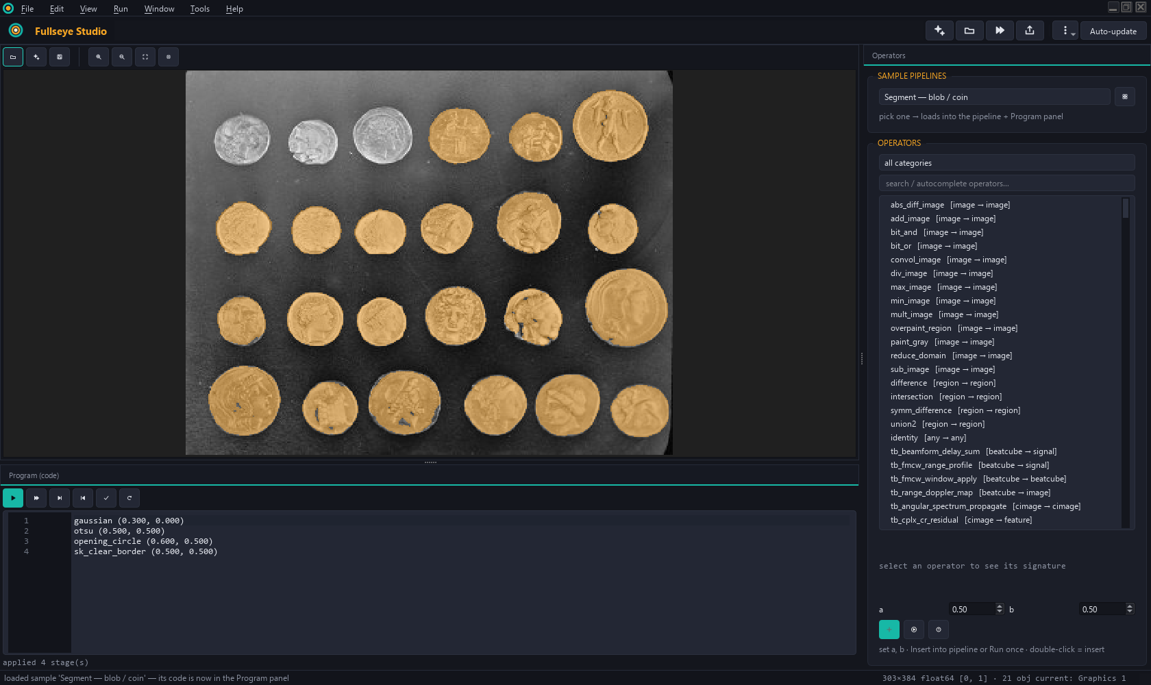
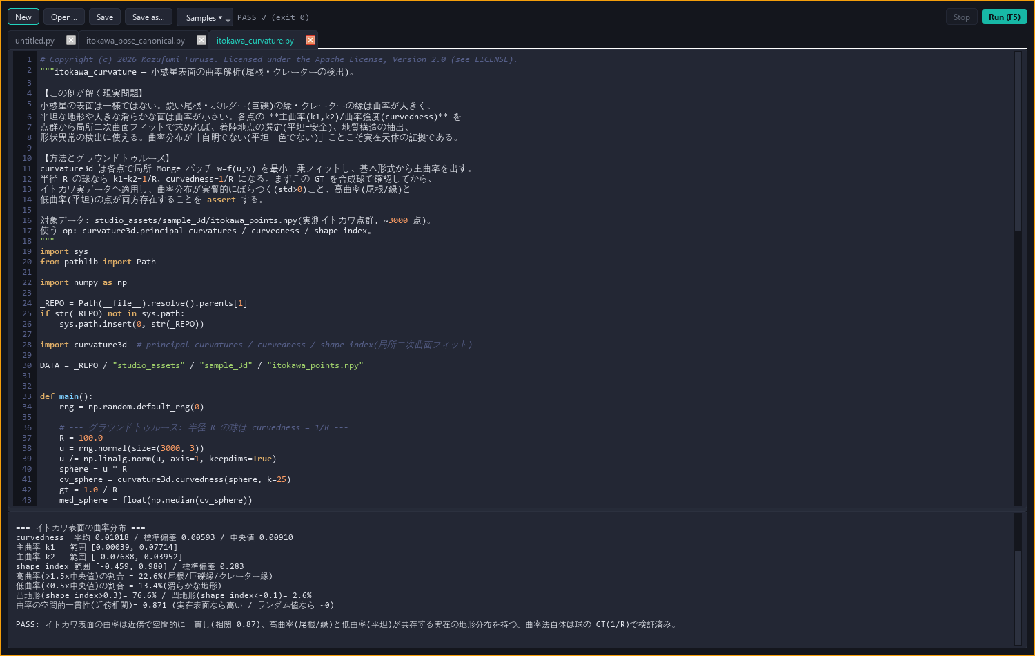
Generated by: tools/gen_studio_screenshots.py. All are real screens headlessly grab()-ed from the
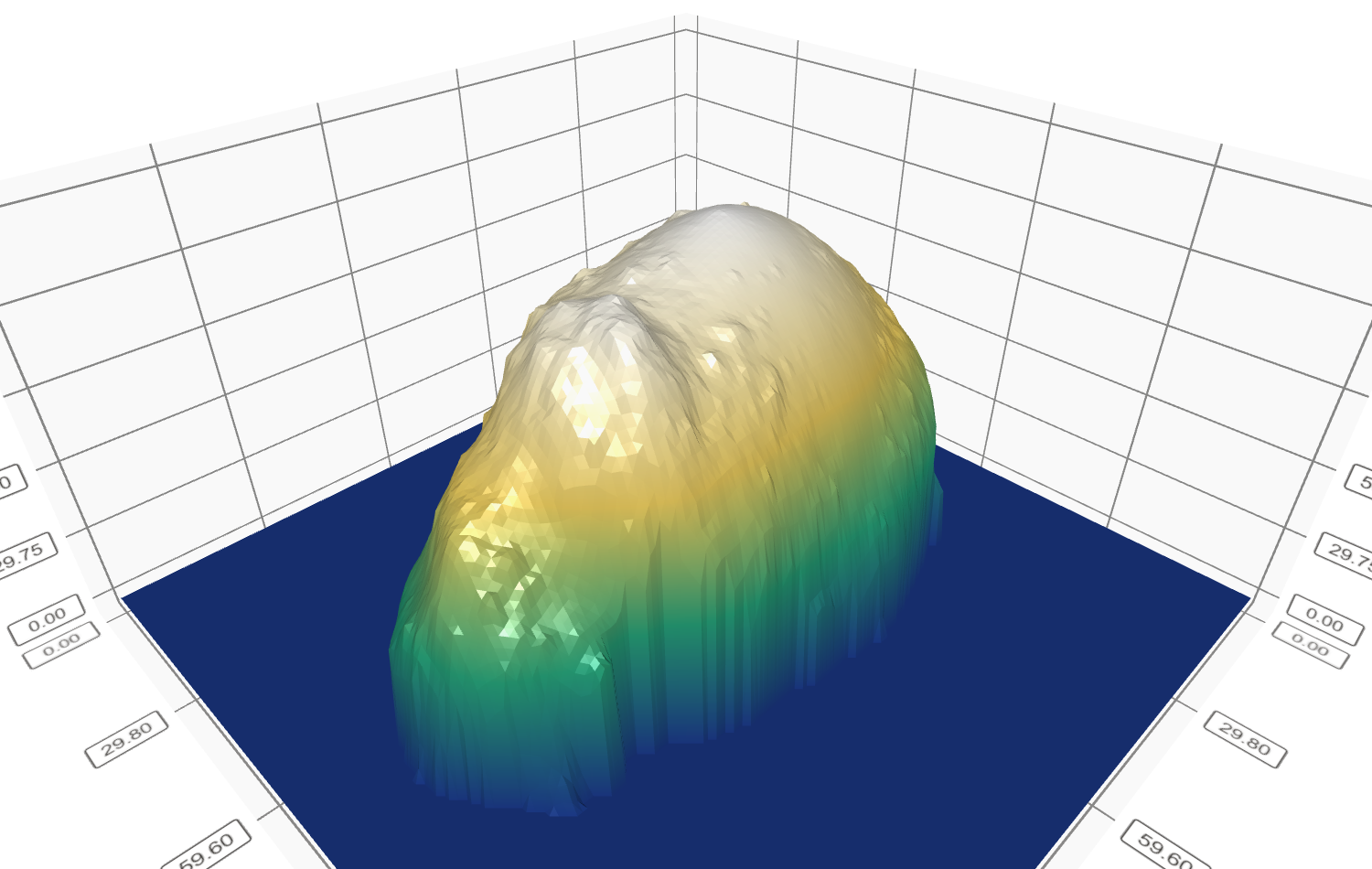
actual Studio UI assembled by studio.build_window() (only the 3D surface uses Q3DSurface.renderToImage
in a real GL context; the series construction shares Studio’s own _build_surface3d_series, built so
that its appearance does not diverge from the real application). There are no mockups.
| Image | Content |
|---|---|
studio_main.png |
The main window. A blob segmentation pipeline (gaussian → otsu → opening_circle → sk_clear_border) is applied to the coins sample image, and 21 coins are overlaid in the region-overlay display. The lower Program panel shows HDevelop-style pipeline code, the right shows the operator browser (search + signature display), and the status bar shows 21 obj |
studio_3d_surface.png |
The rotatable 3-D surface view opened with Ctrl+3 (Q3DSurface, height-linked terrain-style gradient). The data is the real-data relief of the Gaskell shape model of asteroid Itokawa (JAXA Hayabusa), depth-imaged via render3d.render_mesh. In the app, this view can be rotated by mouse drag and zoomed with the wheel |
studio_python_editor.png |
The Python Editor (tabbed, editing multiple scripts simultaneously). Just after opening examples_3d/itokawa_curvature.py and running it with F5, the lower console shows the actual output of the Itokawa curvature analysis (PASS, exit 0) |
studio_3d_examples.png |
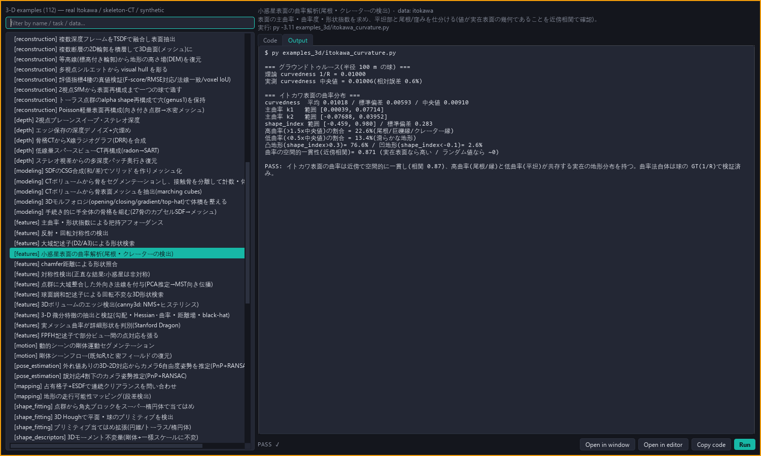
The 3-D Examples gallery (105 real-data worked examples). Just after selecting itokawa_curvature and clicking Run, the Output tab shows the execution result with ground-truth verification (PASS) |
studio_3d_ops.png |
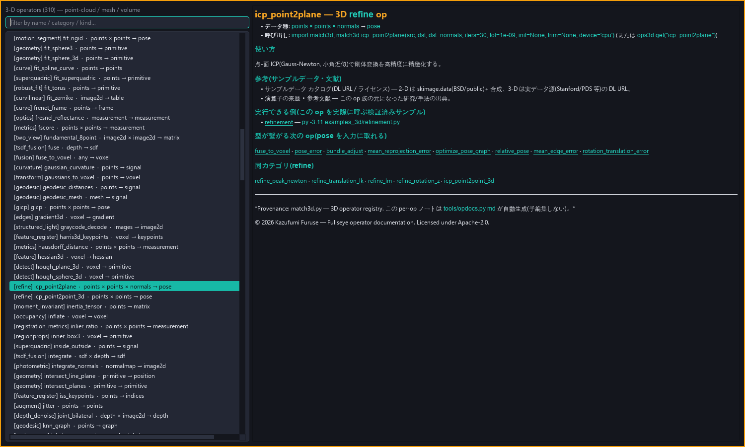
The 3-D Operators reference (265 ops). The generated help page of icp_point2plane (signature, usage, verified samples, links to the next op where the types connect) |
7. Science gallery (science_*.png/gif)
Generated by: tools/gen_science_gallery.py (regenerable per subject:
py -3.11 tools/gen_science_gallery.py --subjects <name,...>).
All are real outputs of fullseye’s registered ops / facade, with no mockups.
Images derived from simulation state that fact explicitly in the caption.
Thumbnails (720px-wide JPG) are the *_thumb.jpg in the same directory.
| Image | Content (ops used / data) |
|---|---|
science_distance_ripple.png |
The distance transform of a real coin photo rendered with rainbow colors and ripple contours (otsu, fill_up, distance_transform / skimage.data coins) |
science_fourier_stars.png |
The FFT spectrum of a real camera photo and a woven texture. The weave lights up like a constellation (fft_image; only the weave panel is synthetic) |
science_watershed_foam.png |
24 coins color-separated one by one with watershed (watersheds, segment_objects, colorize_labels) |
science_edge_compass.png |
A neon image painting contour orientation with a hue wheel (sobel_dir, sobel_amp) |
science_alife_worlds.png |
6 panels of Rule 90 fractal / Rule 30 chaos / sandpile / DLA dendrite / Lenia / cyclic CA (iterated application of alife_*. Simulation images) |
science_dino_xray.png |
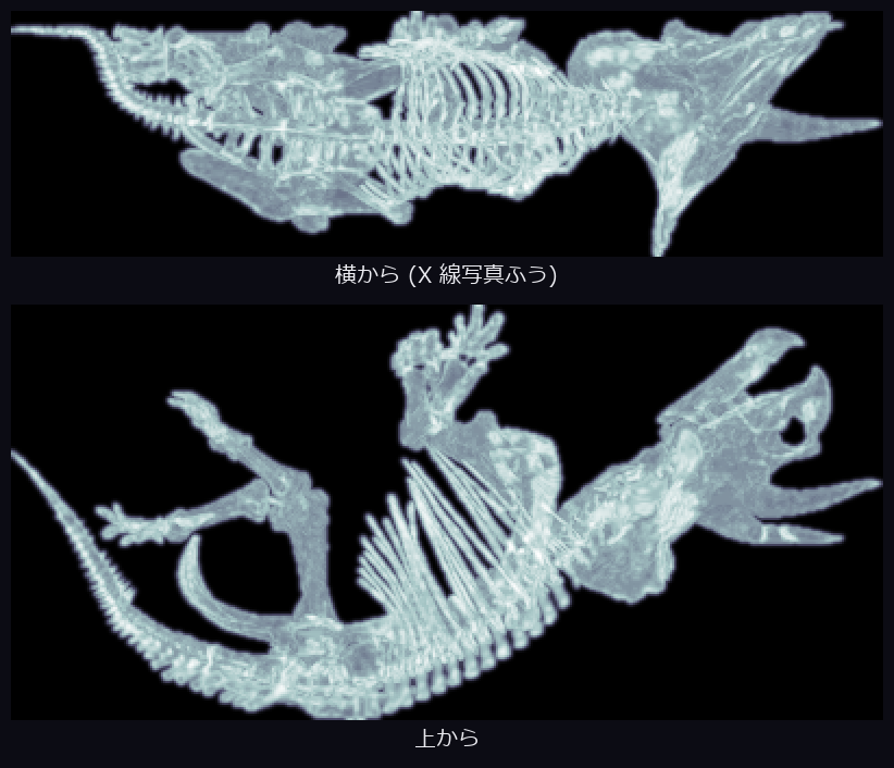
A real scan of the Smithsonian Triceratops osteological specimen (CC0), voxelized → an X-ray look via vol_mip (voxelize, vol_gaussian, vol_mip) |
science_dragon_anaglyph.png |
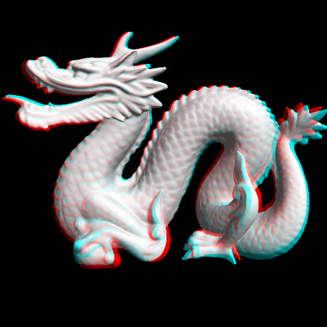
A red-cyan anaglyph of two-viewpoint renders of the Stanford dragon (read_mesh, look_at, render_mesh) |
science_dino_terrain.png |
A 600k-point cloud of the osteological specimen → elevation map → terrain-shading coloring. The spine becomes a mountain range (elevation_map, colorize_height) |
science_morph_pulse.gif |
A 26-frame morphology animation: merging by dilation → thinning by erosion (dilation_circle, erosion_circle) |
science_wobble_warp.png |
Before/after of spatial deformation in the 3 styles of TPS/FFD/MLS (deform_tps/ffd/mls) |
science_dino_skeleton.png |
Extracting the centerline in gold from the top-down silhouette of the osteological specimen (sk_skeleton) |
8. Cross-discipline gallery (academic_*.png)
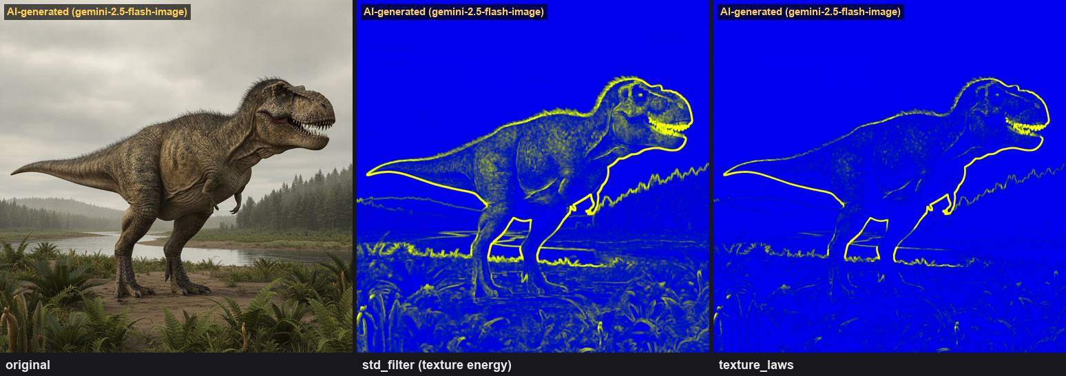
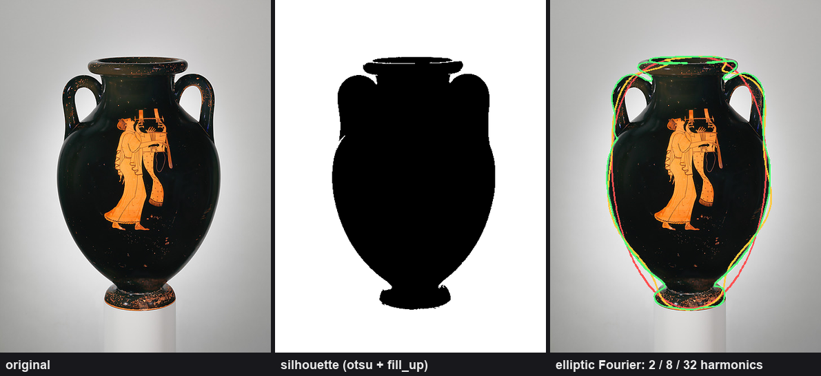
Generated by: tools/gen_academic_gallery.py. 30 exhibits = 8 real data + 22 AI-generated.
It covers medicine, archaeology, biology, space, paleontology, geology, meteorology, oceanography, and
botany, with every image structured as a before → after pair with fullseye’s registered ops applied.
- Real data uses only the Smithsonian (CC0), the Metropolitan Museum of Art (CC0), and NASA (public domain). For the source and license of every asset, see the attribution table in articles/assets/ACADEMIC_ATTRIBUTION.md.
- The AI-generated (Google gemini-2.5-flash-image) mock data is stamped with “AI-generated” in the top-left of every panel of the montage, and also noted in the attribution table (these are not real specimens, patients, or scans).
- This collection and processing also serves as bug discovery through real data, and the 5 issues found are recorded in KNOWN_ISSUES.md.
Two representatives (for all 30, refer directly to articles/assets/academic_*.png):
9. Industrial + Physical AI gallery (industrial_*.png / phai_*.png)
Generated by: tools/gen_industrial_gallery.py (--subjects selectable).
All are real processing on synthetic data / MuJoCo simulations, and the detection/measurement results
are confirmed with assert to match the known ground truth (placement count, drawn dimensions,
placement pose).
| Image | Content (verification) |
|---|---|
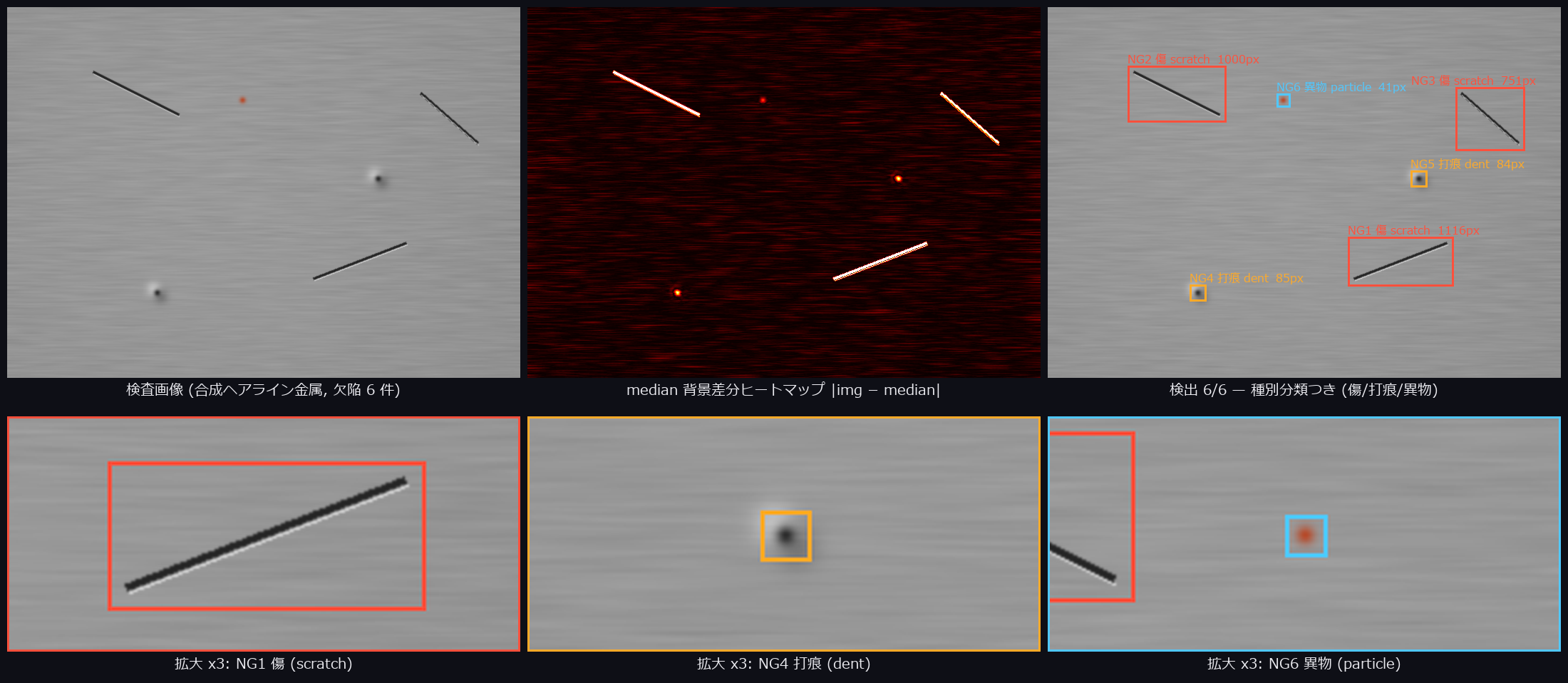
industrial_defect.png |
A hairline metal surface with 3 scratches, 2 dents, 1 foreign object → median background subtraction → red boxes + area (6/6 detected) |
industrial_metrology.png |
Measuring the 3-step diameters of a stepped shaft with a sub-pixel caliper (max error 0.02px) |
industrial_align.png |
Shape-matching localization of 3 rotated workpieces (position 0.0px, angle 0.0° match, no response to a different part) |
industrial_blobs.png |
60 pellets (6 touching pairs) counted with marker watershed 60/60 + size classification into 3 colors |
industrial_barcode.png |
Edge-pair detection of 45 bars (all edges ±1.5px) + scan-line profile |
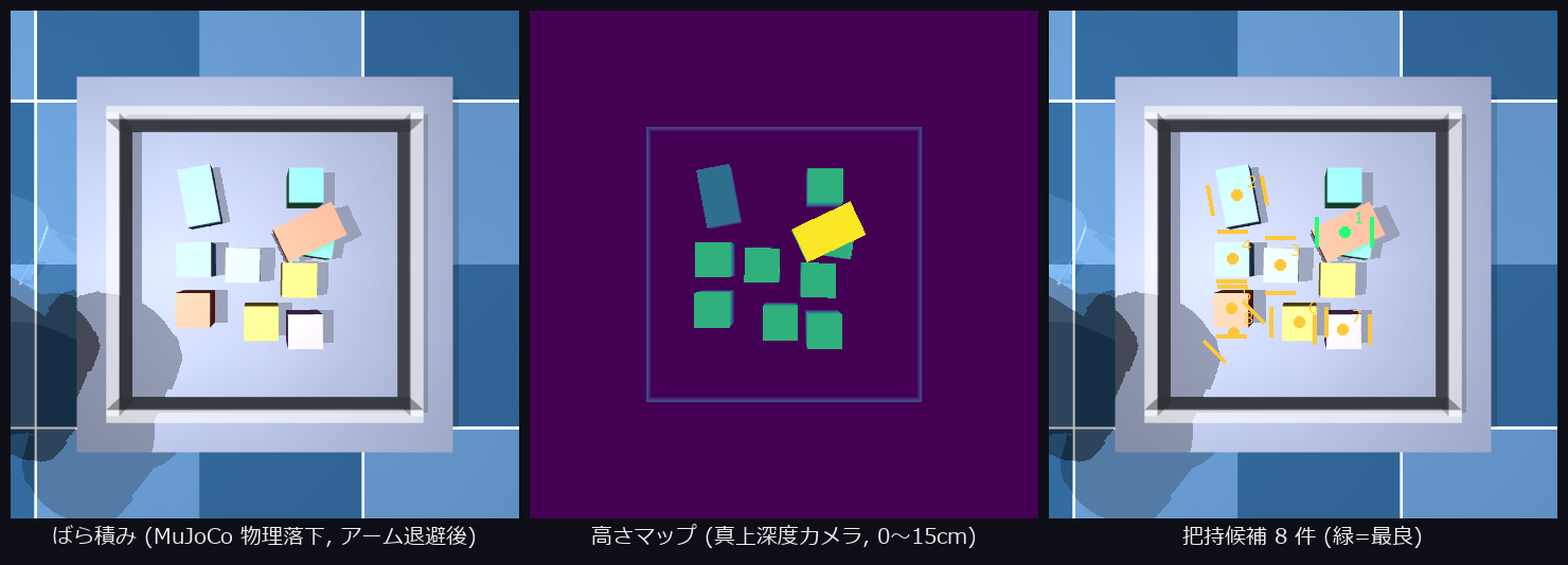
phai_binpick.png |
Bin of parts from MuJoCo physical drop → height map → scoring 8 grasp candidates |
phai_lidar_clusters.png |
23k real ray casts → ground removal → 6 clusters + OBB bird’s-eye view (6/6) |
phai_stereo_obstacles.png |
Disparity → 3D reconstruction → bird’s-eye obstacle map (4/4, median ground error 3mm) |
phai_focus_stack.png |
7 focal planes → all-in-focus composite (sharpness ×1.27) |
media/phai_bin_pick.mp4 |
A full cycle where the Panda picks a grasp candidate, grabs it with 6-DOF IK, and carries it out (150 frames, 3/3 successful outfeed measured) |