fullseye
言語 / Language: 日本語 · English
A Table-Tennis Ball Bounces, So a Tracker That Ignores Physics Misses the Landing Point by 20 cm — A PoC Series That Measures Bounce and Friction from Video
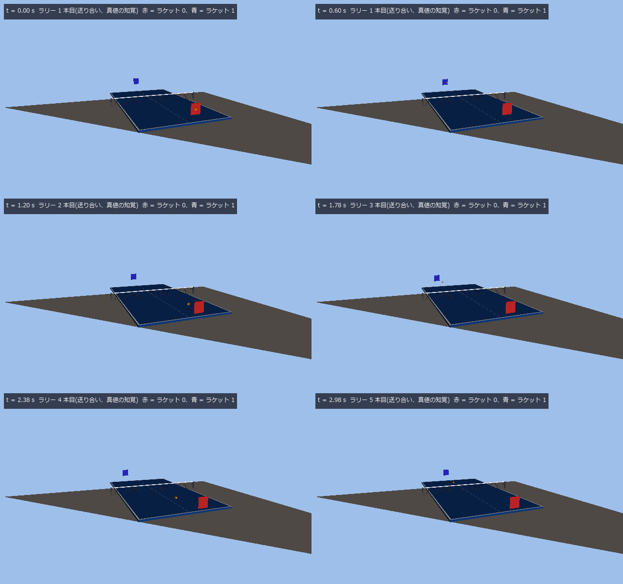
↑ Two freely moving rackets (red, blue) return a ball that bounced once on the opponent’s side, aiming with the equations of motion. First 3 seconds at 1/5 speed. That the rally continued is visible. The point of this article is that the number of hits is a report card for perception, prediction and control at once.
About this article
A table-tennis ball weighs 2.7 g, flies at close to 100 km/h, bounces on the table and spins at 3,000 rpm. Air drag slows it, spin bends its path (the Magnus force), and on the table the spin changes how it bounces. A tracker that follows a parabola is right until the bounce and misses the landing point after it by 20 cm.
Robot table-tennis research triangulates the ball from several high-speed cameras, predicts through the bounce with equations of motion that include drag and Magnus, and measures spin from the ball’s markings. This article builds that whole chain in numpy only, with a gate backed by ground truth at every stage.
(i) Is a theorem the gate, (ii) is a second implementation that assumes no closed-form structure the ground truth, or (iii) is there a published value (a standard, a measurement)? Nothing that satisfies none of these is written. Checking an answer with the formula that produced it is forbidden.
The criteria are the same as in the autonomous-driving series (here). What differs is the subject — things that bounce, slide and spin — so the friction coefficient and the coefficient of restitution take the lead. Kendama (a ball on a string and a cup) uses the same tools, so it continues in this series.
Where the series is
| Part | What is measured | Gates (where the truth comes from) |
|---|---|---|
| 1 | The ball bounces — tracking, triangulation, prediction through the bounce, spin, rally | closed forms in vacuum / angular momentum about the contact point / apex ratio e^{2k}h₀ / the ITTF bounce standard / a world with ground truth / the rally length |
| 2 | Kendama — the string only pulls, the ball flies a parabola, the cup is carried by a prediction from images | elliptic integral and period theorems / closed forms of tension and slack angle / Japan Kendama Association dimensions / a world with ground truth / 3DGS projection and compositing formulas |
| 3 | Filming a spinning ball and reading its spin two ways — from the curve and from the markings | the ω × v theorem (spin about the direction of travel produces no force) / a world with ground truth / two independent readings (track and markings) agree |
| 4 | Filming a bouncing ball with a high-speed camera and reading restitution and friction — checked against published values | the closed forms of Cross 2002 / the ITTF table bounce / the speed dependence of restitution in Inaba et al. 2017 / a world with ground truth |
| 5 | Reading errors end the rally — how much noise and latency move the landing point, in closed form before the shot | the closed-form error propagation in a vacuum / first-order propagation J Σ Jᵀ / the binomial distribution / latency under constant acceleration |
Part 1: The ball bounces — tracking, triangulation, prediction through the bounce, spin, rally
Procedure
Dynamics : drag (Reynolds-dependent sphere model) + Magnus (spin ratio) + spin decay + speed-dependent restitution + Coulomb bounce (grip / slip), integrated with RK4
World    : an ITTF table (2.74 × 1.525 m, 0.76 m high, net 15.25 cm) and a 40 mm ball (14 black markers) with ground truth. Two tracking cameras + one close-up camera at the bounce
Video    : detect the ball by chromaticity (sub-pixel) → track with constant-velocity prediction → DLT triangulation → constant-acceleration Kalman
Predict  : detect the bounce at a local minimum of z → fit 6 parameters of the equations of motion by Gauss–Newton to the 15 frames before it → read the landing point through the bounce
Measure  : restitution e from fits to 12 frames on each side; angular velocity from marker correspondences (Kabsch) on the close-up camera
Rally    : two rackets meet the ball after one bounce on the opponent's side and return it to a chosen point. Before each hit they look ahead and rewind if the shot would fail. The hit count is the metric
In plain words: three formulas decide the motion. Drag (the faster, the stronger the deceleration), the Magnus force (the ball curves in the direction of spin × velocity), and the bounce (the vertical speed comes back scaled by e, the horizontal speed is trimmed by friction, and the spin changes). Tracking finds the ball in the images and puts it back into 3-D; prediction integrates the formulas; measurement is the inverse problem.
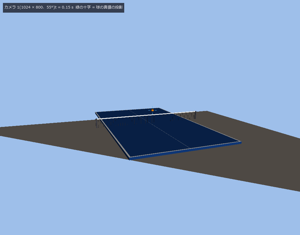
↑ Tracking camera 1 at t = 0.15 s. The ball is only 4 px in radius. The cross is the projection of the world’s own ground truth.
Gates and scores
| # | Gate | Truth | Score |
|---|---|---|---|
| 1 | Identities in vacuum | closed form | RK4 vs closed form 1e-12; a parabola fit returns g = 9.81 to 4e-15 |
| 2 | Bounce theorems | angular momentum about the contact point | 500 random impacts (e ∈ [0.3, 1], μ ∈ [0, 0.6]): relative error at most 4.9e-16, energy never increases, 136 switch to rolling / 364 keep slipping |
| 3 | Apex ratio and the ITTF bounce | e^{2k}h₀ and the 24–26 cm standard | dropped from 30.5 cm: apexes 24.7 / 20.0 / 16.2 / 13.1 cm, 3e-7 from the closed form; total time 4.736 s (closed form 4.738 s) |
| 4 | Detection | projected world truth | 122 / 122 frames, median centre error 0.15 px (image radius 4.3 px) |
| 5 | Triangulation | world truth | 4e-15 m from projected truth, median 1.6 mm from detections |
| 6 | Kalman | a parabolic truth | innovation at most 8e-9 m (2e-3 m with drag and Magnus in the truth = outside the model); median velocity error 0.07 m/s |
| 7 | Bounce detection | the world’s contact time | 0.6 ms off (one frame = 10 ms) |
| 8 | Prediction through the bounce | the world’s landing point | 0.4 cm with the true spin, 20.2 cm ignoring spin, 6.6 cm with a parabola |
| 9 | Spin | the world’s angular velocity | markers matched in 19 / 19 frame pairs, relative error 3.7 % at |ω| = 2394 rpm |
| 10 | Restitution | the world’s e = 0.90 | 0.911 from equation-of-motion fits; 0.940 from parabola fits (drag and Magnus absorbed into g) |
| 11 | Rally length | the cap, an attacker, perception noise | feeder vs feeder 12 (cap), attacker vs feeder 9 (out), perception noise 0 / 50 / 100 mm → 8 / 8 / 2 hits |
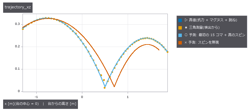
↑ Points triangulated from detections (median error 1.6 mm) sit on the truth. Reading ahead from the state fitted to the 15 frames before the bounce, the landing point is 0.4 cm off if the 2291 rpm topspin is known, and 20.2 cm off if spin is ignored.
How to read gate 11 (the claim of this article). The rally length grows only when detection, triangulation, prediction, shot planning and racket motion are all right at the same time. If any one stage breaks, it shows in the count, so one number scores the chain. Make one side “play to win” (fast to the far corner) and the rally ends at 9; make both sides “return close to last time, shifted a little” and it runs to the cap. Adding 5 cm of noise to perception does not shorten the rally; 10 cm drops it to 2. The flat part is the slack of the racket face (15 × 16 cm) — errors smaller than half the face do not show in the count, which is also the resolution of the metric.
Rewinding. Before each hit, the planner looks ahead with the true physics; if the shot would hit the net, bounce on its own side or arrive at an unreachable height, it rewinds time and tries again (counted). The attacker still ends at 9 hits after 99 rewinds because the mismatch between the planner’s formulas (a closed-form aim plus iteration) and the world’s physics (Reynolds-dependent drag, spin-ratio lift) grows with ball speed. The rewind count can be read as the amount of mismatch between planner and physics.
★ Where implementations go wrong
1. Gate the Kalman filter on a real trajectory and it looks broken
A constant-acceleration Kalman filter is exact for a parabola (innovation 1e-9 m). Feed it a trajectory with drag and Magnus and the innovation is 2e-3 m — that is being outside the model, not a defect in the filter. Gate it on a parabola, and give the real trajectory to the equations of motion for prediction.
2. Fit a parabola and the restitution is 4 % off
Fitting parabolas before and after the bounce to get v_z absorbs drag and Magnus into gravity: e = 0.940 (truth 0.90). Fitting the equations of motion gives 0.911. The landing point behaves the same way: 6.6 cm with a parabola, 0.4 cm with the equations. Fit with the same equations you predict with.
3. One marker does not determine the rotation
Knowing one marker’s direction says nothing about rotation around that axis. Kabsch (least-squares rotation from two or more direction pairs) needs at least two markers visible in the same frame pair. With markers on six axes only, 2–3 are visible and some merge with the dark rim into one. With 14 markers (6 axes + 8 corners) and strobe-like lighting on the close-up camera (weak shading), 19 / 19 frame pairs match.
4. A moving racket bounces in relative velocity
| The racket face moves, so putting the ball’s velocity straight into the bounce formula is wrong. Subtract the face velocity, bounce, add it back. The closed-form aim is the same: n ∝ v_out − v_in and v_r·n = | Δv | / (1 + e) + v_in·n. |
5. Bounded motion overshoots the acceleration limit in the last step
Bang-bang motion (full acceleration, then full braking just in time) run in discrete time exceeds the acceleration bound in the step before stopping. Use max(0, √(2ad) − a·dt) for the stopping speed to keep one discrete step of margin.
6. Bounces never end (Zeno)
Apexes follow e^{2k}h₀, the intervals shrink geometrically, and infinitely many contacts fit inside the total time √(2h₀/g)(1 + e)/(1 − e). Unless you decide to put the ball on the table once the vertical contact speed drops below a threshold, the integration never stops.
7. A zero normal spreads NaN silently
If normalising by a zero length returns NaN instead of raising, the rest of the rally is NaN and counts as “continued”. Fail closed (ValueError); the gates do not let NaN through.
What it is not for
No real video yet. Cameras, table and ball are a synthetic world with ground truth. The chromaticity detector is robust to shading but will pick up anything of the same chromaticity in the background. Real footage is a later part.
The default drag and lift coefficients are literature values, not measurements. There is an identification op (fit_aero: Gauss–Newton for C_d and C_L from a trajectory, recovers the truth to 1e-15), but it has not been run on a real ball.
The rally planner knows the world’s physics. Rewinding uses the true physics to look ahead, so it does not transfer to a real machine as is. On a real machine the predictor (equation-of-motion fits) would do the look-ahead, and rewinds become “the gap between what the predictor said and what happened”.
Spin measurement needs markers. Kabsch cannot stand on a plain ball. Using the seam or the logo is a different op.
Run it
git clone https://github.com/furuse-kazufumi/fullseye
cd fullseye
py -3.11 examples/poc_ball_bounce.py            # 11 gates and 8 figures (2 GIFs), about 110 s
import numpy as np
import fullseye as fs

bp = fs.ledger.ball_params()                      # 40 mm, 2.7 g, drag 0.4, lift from the spin ratio
ip = fs.ledger.impact_params(0.90, 0.25)          # restitution e, friction μ
tp = fs.ledger.table_params()                     # ITTF: 2.74 × 1.525 m, 0.76 m high

# a topspin shot over the table (table at z = 0.76, bounces only inside its outline)
r = fs.ledger.flight_simulate([-1.3, 0.0, 1.0], [5.2, -0.3, 0.6], [0.0, 240.0, 0.0], bp, ip,
                              t_end=0.8, table_z=tp["height"], table_xy=(-1.37, 1.37, -0.7625, 0.7625))
c = r["contacts"][0]
print(round(c["t"], 4), np.round(c["p"][:2], 3), c["regime"], np.round(c["omega_out"], 1))
# 0.2495 [-0.095 -0.07 ] grip [  7.8 228.8   0. ]     ← contact time [s], point [m], grip or slip, spin after the bounce [rad/s]

# drop from 30.5 cm: apex ratio and the ITTF standard (first bounce 24–26 cm)
h = fs.ledger.apex_sequence(0.305, 0.90, 4)              # h₀ and the next 4 apexes
print(np.round(100 * h, 1))
# [30.5 24.7 20.  16.2 13.1]

# two rackets, up to 12 hits (feeder vs feeder)
rp = fs.ledger.racket_params()
from racket import strategy_feeder, strategy_attacker
res = fs.ledger.rally_simulate(bp, rp, tp, strategies=(strategy_feeder, strategy_feeder), retries=0, max_hits=12, seed=1, table_ip=ip)
print(res["hits"], res["end_reason"], res["rewinds"])
# 12 max_hits 0
Look at end_reason: out, net, double_bounce or unreachable. With the attacker it ends at 9 hits with out. When the count drops, it is the ball’s motion, the perception or the planner — read it together with the rewind count and the stage narrows down.
This part produced 8 figures in total — see them all
The remaining figures of this part
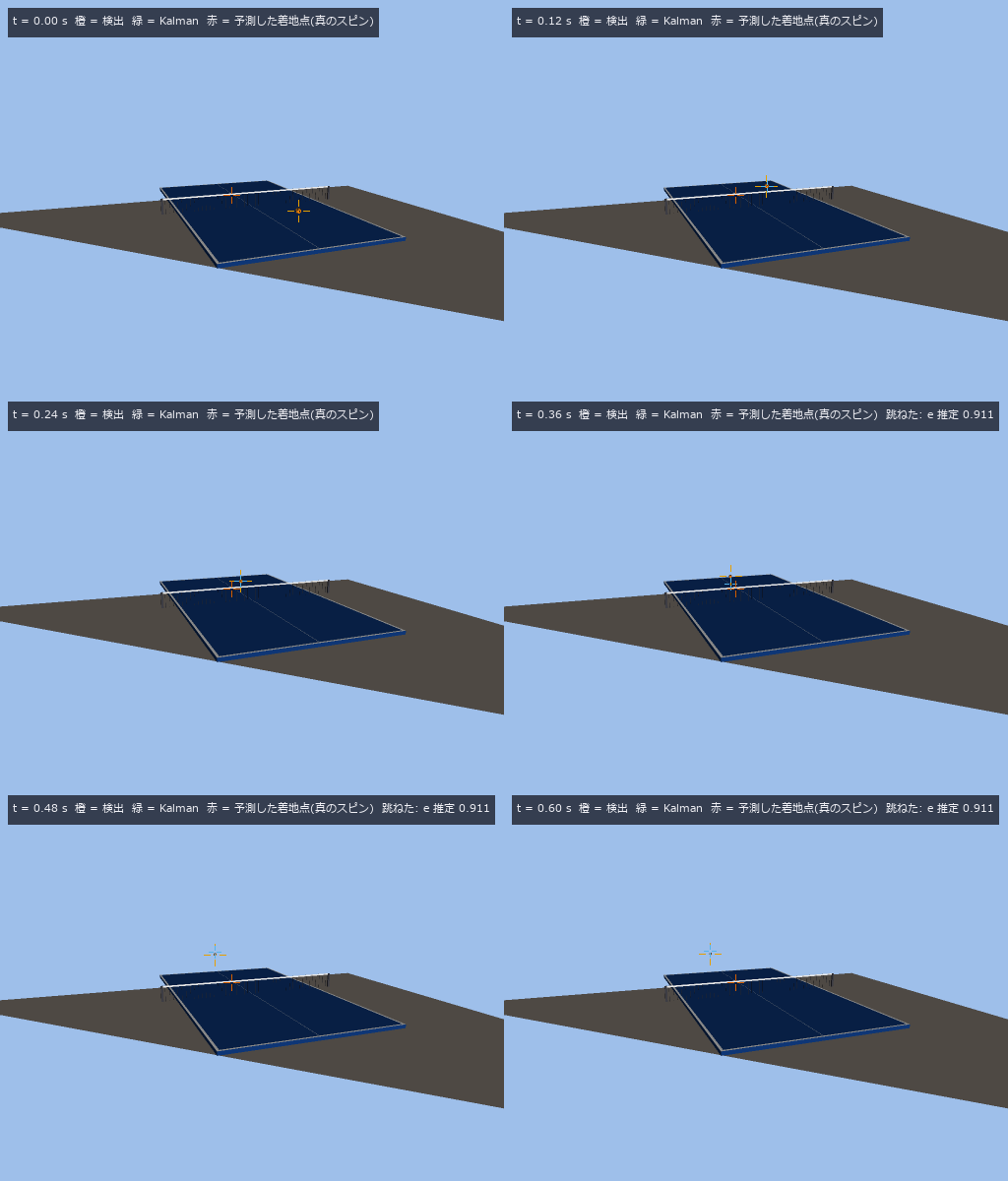
↑ Tracking camera 1, 100 fps at 1/10 speed. Orange crosses are detections, green is the projected Kalman state, red is the landing point predicted from the 15 frames before the bounce.
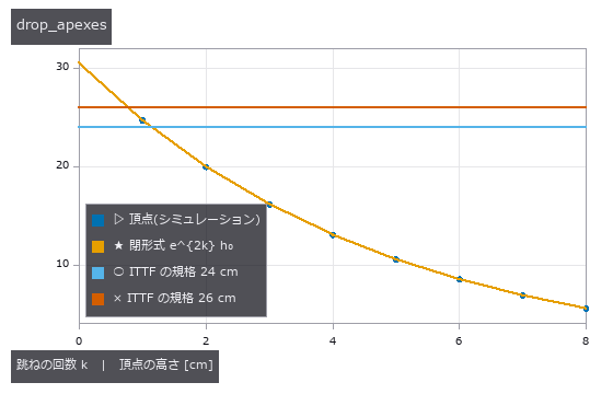
↑ Apexes of a ball dropped from 30.5 cm (e = 0.90). They match the closed form e^{2k}h₀ to 1e-6, and the first bounce of 24.7 cm is inside the ITTF standard of 24–26 cm.
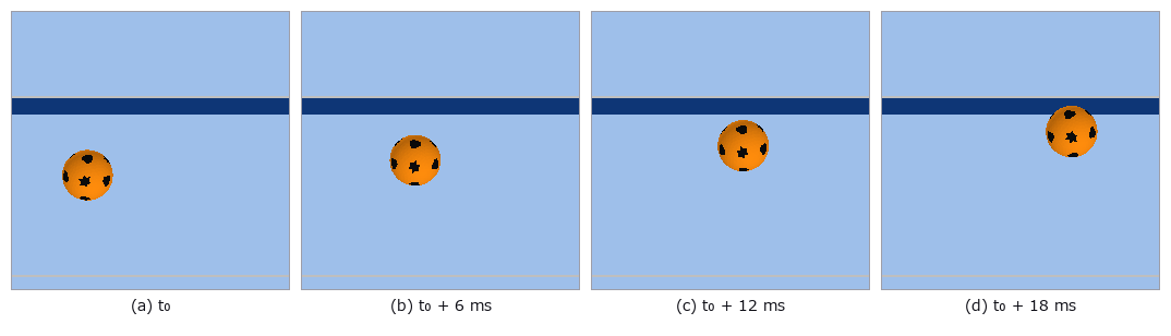
↑ Four frames from the close-up camera at the bounce (1000 fps, 20°). The directions of the visible black markers (4–6 of 14) are matched to the previous frame and the rotation is solved with Kabsch.
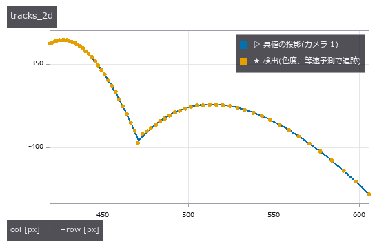
↑ The ball’s track in camera 1’s image: projected truth (line) and detections (points). Median centre error 0.15 px.
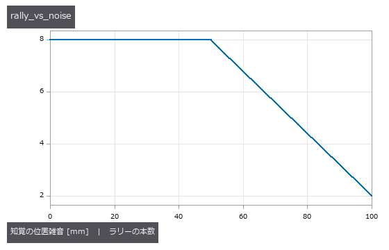
↑ Rally length (feeder vs feeder, cap 8) with Gaussian noise added to the perceived ball position. No loss up to 5 cm, 2 hits at 10 cm. The flat part is the slack of the racket face.
Part 2: Kendama — the string only pulls, the ball flies a parabola, the cup is carried by a prediction from images
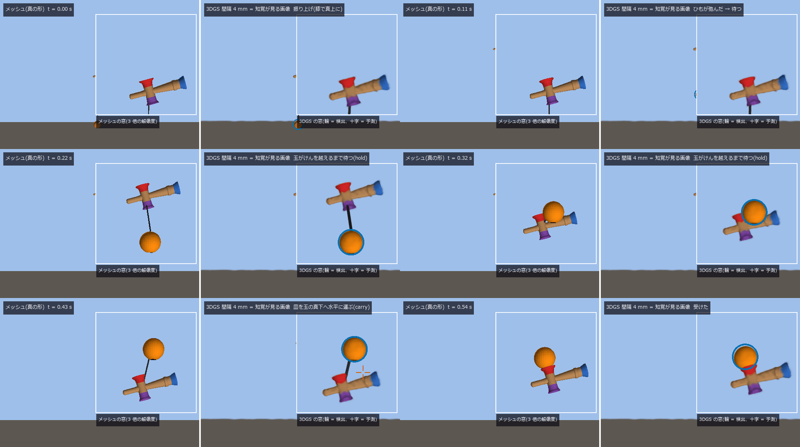
↑ Right = the image the closed loop’s perception actually saw (the world turned into 3D Gaussian Splatting and rendered), left = the true shape at the same moment. The window at top right re-renders the kendama at three times the resolution. Blue ring = the ball found by chromaticity, cross = the landing point read from the parabola fitted to the frames after the string went slack. The only thing that moves the cup is the image on the right.
The basic moves of kendama
From the Japan Kendama Association’s graded tricks, this part takes the four in which the ball is pulled straight up and caught in a cup.
| Trick | Grip | Cup |
|---|---|---|
| Big cup (ōzara) | cup grip (spike tilted down, big cup up) | big cup |
| Small cup (kozara) | same grip | small cup |
| Base cup (chūzara) | ken grip (spike almost straight down) | base cup |
| Candle (rōsoku) | pinch the spike | base cup |
The teachers’ procedure is the same for all: pull straight up with the knees → move the ken only after the string goes slack → carry the cup horizontally under the point where the ball will come down (do not scoop) → bend the knees at touchdown to absorb the impact. This PoC turns that procedure directly into the stages of its controller.
Four rules. (1) Only gravity and string tension move the ball (a one-sided constraint, tension ≥ 0). (2) The ken and the cross piece are one rigid body whose position may move freely. (3) The ball rises after the string goes slack and is caught on the way down after its apex (a straight-up path counts as a parabola). (4) The spike is only for the ball’s hole — in the cup tricks, touching the spike or the cross piece is a failure.
Procedure
Shape      : from the Japan Kendama Association's published values (60 mm ball, 70 mm across, 180 mm assembled) and the JKA 16-2
             description (160 mm ken, cups 42 / 38 / 35 mm), the ken and cross piece are solids of revolution; so is the ball, hole included
             (a 17 mm wide, 40 mm deep cavity)
Mechanics  : string = one-sided constraint tension ≥ 0 (free fall when slack, radial speed lost when it snaps taut), by projection; with drag
World      : two cameras (480 × 360, 100 fps). A synthetic world with ground truth, additionally turned into 3D Gaussian Splatting before rendering
Perception : ball by chromaticity → triangulate from two cameras → "slack" when the ball is closer to the string hole than the string length
             for two frames in a row → fit a gravity-known parabola (6 unknowns)
Control    : lift (straight up with the knees) → wait (do not move until slack) → hold (do not approach until the ball clears the ken)
             → carry (cup horizontally under the landing point) → absorb (lower it at touchdown)
Scoring    : at the moment of touching the rim, lateral ≤ rim radius, relative speed ≤ 1 m/s, descending. Touching the ken = hit_ken (fail)
In plain words: a string cannot push. It can only pull — a “one-sided constraint”. So when the ball is pulled up hard, at some moment the string goes slack, and from then on the ball flies a parabola. A parabola is fixed by gravity alone, so once a few positions after the slack are known, where the ball will come down can be computed. The cup only has to get there first and wait. What a person does as “watch the ball and wait where it falls” is done here with images and a parabola.
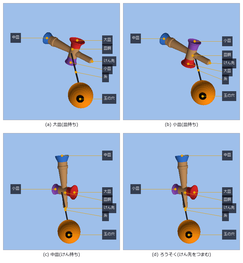
↑ The poses of the four grips. The ken and cross piece are one rigid body; only where it is held differs. Every dimension measured from the vertices matches the published value to 1e-9.
Gates and scores
| # | Gate | Truth | Score |
|---|---|---|---|
| 1 | Elliptic integral and large-amplitude pendulum period | published K(0.5) and the theorem T = 4√(L/g)K(sin θ₀/2) | K error 0; period string 3.0e-4, rod 8.9e-11 |
| 2 | Tension and slack angle | closed forms m(v²/L + g cos θ), cos θ_s = (2/3) cos θ₀ | tension 0.26 %; slack angle 125.04° (closed form 125.26°) |
| 3 | Energy and snap | conserved in flight; loss when taut = ½ m v_r² | spread in flight 2.5e-15 J; snap 0.2362 J vs 0.2367 J; dissipation first order in dt (ratio 9.7) |
| 4 | Shape | published values (70 across, 160 ken, cups 42/38/35, 60 ball, 180 mm assembled) | all 1e-9 |
| 5 | Big cup with true perception | stage order, no contact with the ken, rise after slack, catch descending | caught with 4.22 mm lateral offset; without the dodge the ball hits the cross piece at 0.260 s |
| 6 | Detection → triangulation → slack | world ground truth | median error 0.51 mm; slack detected +23 ms after truth |
| 7 | Closed loop on images only | success rate with true perception | 20 trials: truth 1.00 / images 1.00 (all 390 estimates the plan received came from images) |
| 8 | Same plan, 3 tricks + candle | flight and contact with the ken | small cup 1.00, base cup 0.95, candle (truth) 0.95; lowering at touchdown cuts relative speed 0.91 → 0.61 m/s |
| 9 | Prediction error | ball position at the catch | 10.51 → 0.98 mm from 3 to 44 frames after slack |
| 10 | Pixel noise | success rate | 1.00 for 0–2 px, 0.90 at 8 px, 0.40 at 16 px |
| 11 | Hole direction (stationary ball) | true hole axis | seen by both cameras in 14 of 40 poses, median error 1.8° |
| 12 | Recommended model (49 mm big cup) | JKA model’s success rate | 1.00 vs 1.00 |
| 13 | Closed loop in a 3DGS world | true perception | on 3DGS images at 4 mm spacing alone, all 1 + 2 trials caught; median triangulation error 0.30 mm |
| 14 | 3DGS knobs | detection rate | 1.00 for spacing 2–64 mm; 0.25 at 20 mm position error; 0.00 at colour error 0.3 |
| 15 | The hole on 3DGS | true hole axis | 1 of 40 poses at 480 × 360; 16 (median 2.3°) at twice the resolution and 2 mm spacing; 0 at 4 mm |
| 16 | 10 consecutive tricks (moshikame, three cups) | toss apex v²/2g, no contact with the kendama, rise then descend | both 10 in a row on images alone (grade 5), relative speed 0.41–0.48 m/s |
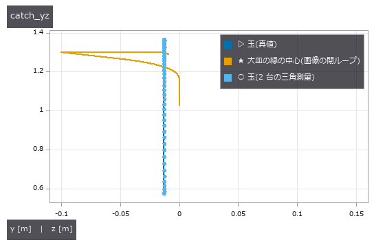
↑ The ball rises after the string goes slack; the cup waits until the ball clears the ken, returns horizontally, drops just before touchdown and catches. Dots are the two-camera triangulation.
Reading gate 9. A parabola fitted to the first 3 frames after slack misses the catch position by 1 cm — the triangulation error rides on the velocity of a short interval. The error falls as frames accumulate and drops below 1 mm at 44 frames. The cup is re-carried to each new prediction every frame, so a wrong first prediction is still in time — the big cup’s rim radius, 21 mm, is the room for “waiting”. Gate 10 staying at 1.00 up to 2 px of pixel noise is the same room; meanwhile the lateral offset grows 2.4 → 4.1 mm.
Recognising after turning the world into 3DGS
Rendering the synthetic world’s meshes directly gives images that are “too clean”. A real scene reconstructed with 3D Gaussian Splatting (3DGS) is blurred in shape and carries errors in position and colour. So a layer was added that turns the world into 3DGS before rendering and feeds the result to the same image processing (gsplatnp, numpy only).
Gaussians : attached to the world's faces (face index + barycentric coordinates + an error fixed in the face's local frame); they follow the vertices
Size      : σ = spacing (the 3DGS initial value). σ ≤ 0.5 R so a disc does not stick out of a curved surface; faces touching an edge (cup rims, the hole's mouth) get 1/4
Rendering : EWA projection Σ' = J W Σ Wᵀ Jᵀ + 0.3 I, front-to-back alpha compositing, Mip-Splatting's opacity compensation
Knobs     : spacing (density), position error, colour error
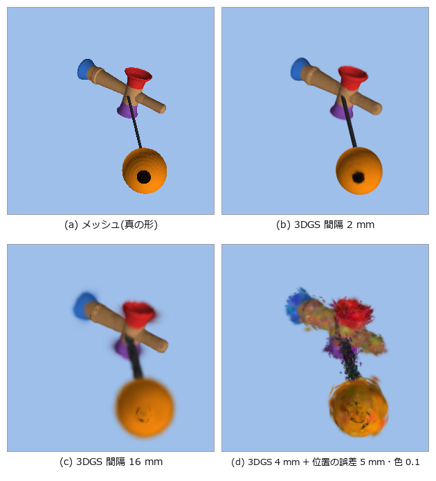
↑ The same close-up camera: mesh and 3DGS (2 mm, 16 mm spacing, with errors). Coarse spacing blurs; errors make it fuzzy with bleeding colour.
The renderer’s gates are three formulas: the second moments of one Gaussian’s alpha image equal Σ’ (and equal the covariance of 3-D samples projected by a separate projection routine); a pixel covered by two Gaussians has the colour of the front-to-back compositing formula (and the image is the same in either array order); moving the world rigidly moves the Gaussians by the same transform.
The results are rows 13–15 of the table. For following the ball, 3DGS hardly matters — even at 64 mm spacing ball detection stays at 1.00 (the curvature cap keeps at least 146 Gaussians on the ball). What breaks it is position error and colour error: with chromaticity detection, a colour error beyond the detector’s tolerance (0.12) makes the ball disappear. The hole is different.
| Poses where the hole was read (of 40) | Mesh | 3DGS 2 mm spacing | 3DGS 4 mm spacing |
|---|---|---|---|
| 480 × 360 | 14 | 1 | — |
| twice the resolution | 23 | 16 (median error 2.3°) | 0 |
At 480 × 360 the ball is 17 px and the hole 5 px. The 3DGS blur (about 1 px) comes in from both sides and fills the hole. Reading the hole needs pixels on the ball and Gaussians inside the hole. To do spike tricks (the spike into the hole), the cameras must sit on the better side of the bottom-right of this table.
Catching in another cup, one after another (consecutive tricks)
After a catch, carry on from that state and catch in another cup: the association’s graded trick moshikame (big cup and base cup in turn) and the three-cup sequence big → small → base.
Toss     : accelerate the cup holding the ball upwards and stop it harder than g → the ball leaves when the cup decelerates faster than it (apex = v²/2g at release)
Turn     : in flight, rotate the ken and cross piece (one rigid body) to bring the next cup up (wrist ≤ 30 rad/s, assumed)
Catch    : carry the next cup under the landing point and move it with the falling ball to match its speed (a hand controller that targets position and velocity)
Perceive : the "flight start" from the cup is also found from images (two frames in a row 12 mm away from the cup seat) → parabola → next cup
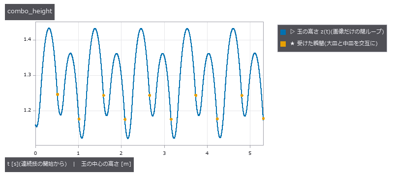
↑ Ball height over 10 moshikame catches in a row (image-only closed loop). It rises and falls on a parabola and is caught by the next cup after the turn. The small dip after each catch is the cup moving with the ball to match its speed (the knees’ cushion).
On images alone, moshikame and the three cups both run 10 in a row (grade 5 on the association’s moshikame table), relative speed at touchdown 0.41–0.48 m/s. A hand controller that targets only position catches nothing with the apex 20 cm above the cup — the cup tries to stop at its target and cannot match a ball arriving at 1.9 m/s. A person “catching with the knees” is a velocity-matching controller.
Honestly: without noise, 100 in a row is the same cycle repeated (the toss is fixed by a closed form and the ball goes straight up), so the count is no evidence of robustness. With 2 px of pixel noise moshikame breaks after 3 and the three cups after 6 (the target jitters with every refit just before touchdown).
★ Where implementations go wrong
1. Adding perception does not mean it feeds the controller
It happens that the parts which triangulate from images and fit a parabola exist, while the plan that moves the cup is still handed the world’s true (p, v). The prediction is only used for scoring, and the closed loop never looks at the images. Gate it as “number of estimates the plan received = number of estimates that came from images” (rows 7 and 13).
2. A string cannot stay taut above 109.47°
Gate the period of a pendulum released from rest at “string, 120°” and it fails. Above θ₀ = 90° the tension is negative from the start, and even launched from the bottom the string goes slack at cos θ_s = (2/3) cos θ₀. Measure large-amplitude periods with a rod, and give the string a slack-angle gate.
3. Without a dodge, a ball rising from straight below hits the cross piece
Pulled straight up, the ball rises from directly beneath the kendama. Left alone it passes through the cross piece (the physics does not resolve the collision, so it passes silently). Measure the ball–kendama gap every step and count contact as failure, and in the second half of the lift move the hand 10 cm towards the string hole. Dodging the other way let the ken hide the ball from a camera and worsened the prediction.
4. Deciding “slack” on one frame fires while the string is taut
Judging “the ball is closer to the string hole than the string length” on a single frame reports slack while taut under 2 px of pixel noise. Require two frames in a row.
5. A hole made as “a dark disc on the surface” vanishes in 3DGS
On a mesh a disc looks like a hole. 3DGS sorts Gaussians by the depth of their centres, so from an angle the ball’s own Gaussians in front cover a disc floating 0.3 mm above the surface, and the hole was read in 0 of 40 poses. Make it what it really is: a 40 mm deep cavity (dark walls and bottom).
6. Gaussians thinner than a pixel get fat unless compensated
Adding 0.3 px² to the 2-D covariance for antialiasing makes sub-pixel Gaussians (the string, cup rims) stay opaque while growing to 0.55 px or more (the string rendered 3 pixels wide). Scaling opacity by √(det Σ / det(Σ + 0.3 I)) (Mip-Splatting) preserves the sum of alpha (gated).
What it is not for
This is not real video. It is a synthetic world with ground truth. The 3DGS is not learned from photos either; it is built from the true shape and degraded with error knobs. It is a tool to measure “does image processing work on the 3DGS representation and renderer”, and it claims nothing about reconstruction quality itself.
The ball’s rotation is not solved. The rendering convention is that the string hole faces the knot while taut and the ball keeps its last pose once slack. The hole direction in flight is not ground truth, and spike tricks are not in yet.
A catch is a geometric test. Bounce and rolling on the rim are not handled; relative speed ≤ 1 m/s is an assumed threshold. The 15° tilt of the cup grip, the cup depths and the 75 g ball are assumptions. The JKA 16-2 dimensions come from a user-supplied description; the primary source was not checked.
Why the candle is harder than the base cup cannot be expressed. The ken moves as a rigid, translating body, so the weak support of pinching fingers is absent, and the numbers come out as the same relative motion as the base cup.
Run it
py -3.11 examples/poc_kendama.py # 16 gates (about 171 s without figures)
import numpy as np
import fullseye as fs

kp = fs.ledger.kendama_params(trick="ozara")          # JKA 16-2 model, big cup (cup grip)
print(round(np.degrees(fs.ledger.tether_slack_angle(np.radians(150.0), kp["pendulum_length"])), 2))
# 125.26                                               ← launched from the bottom with the energy of 150°, the string goes slack here

w = fs.ledger.kendama_world(kp)                       # world with ground truth (ken, cross piece, ball, string)
gs = fs.ledger.gs_from_world(w, spacing=0.004)        # turn the world into 3DGS (4 mm spacing)
rig = fs.ledger.kendama_rig(kp)                       # two cameras
c = rig[0]
img = fs.ledger.gs_render(gs, c["pose"], c["K"], c["width"], c["height"])["color"]
print(img.shape)
# (360, 480, 3)
Set trick in kendama_params to "kozara" / "chuzara" / "rousoku" and only the grip changes, with the same plan. With camera_perceiver(world, rig, render_fn=fs.ledger.gs_render_fn(gs)) the closed loop’s perception looks at 3DGS images.
This part produced 11 figures in all — see them all
The remaining figures of this part
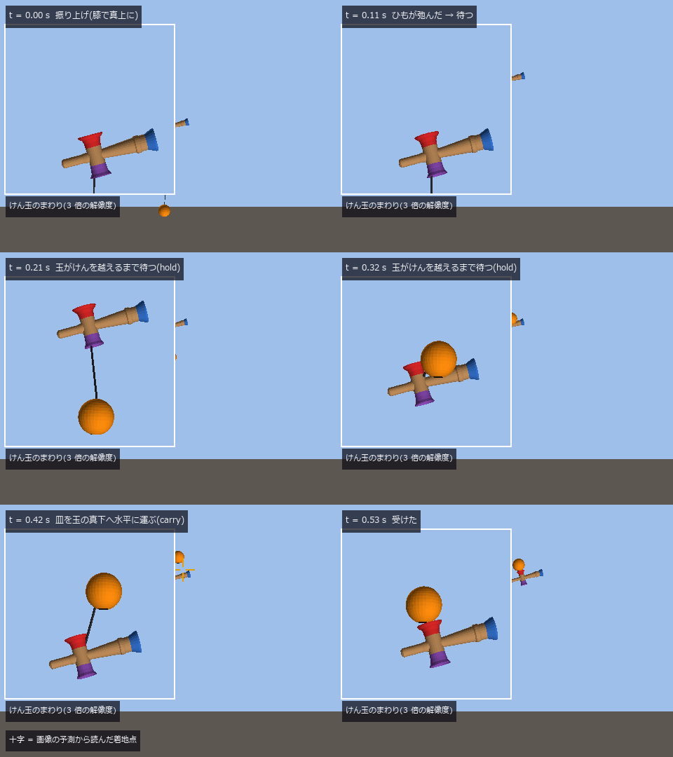
↑ The image-only closed loop in the mesh world (camera 2, 100 fps at 1/10 speed). The cross is the predicted landing point.
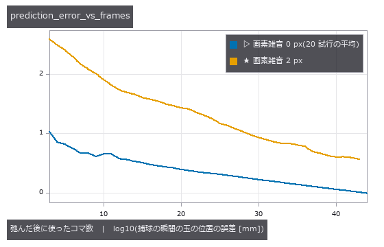
↑ Error of the position at the catch read from the parabola fitted to n frames after slack (log10 mm on the vertical axis).
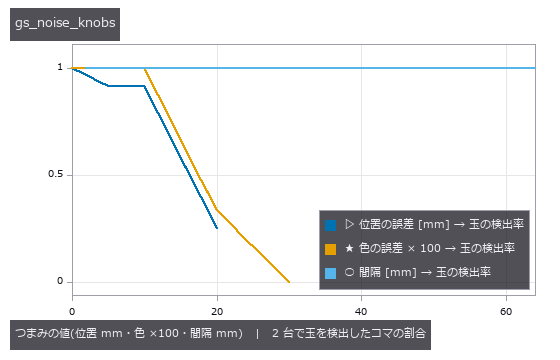
↑ 3DGS knobs and ball detection rate. Spacing does not matter; position and colour errors do.
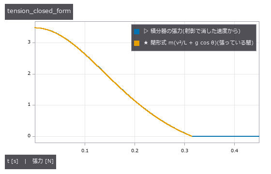
↑ The integrator’s tension and the closed form m(v²/L + g cos θ). The string goes slack at the angle where it reaches 0.
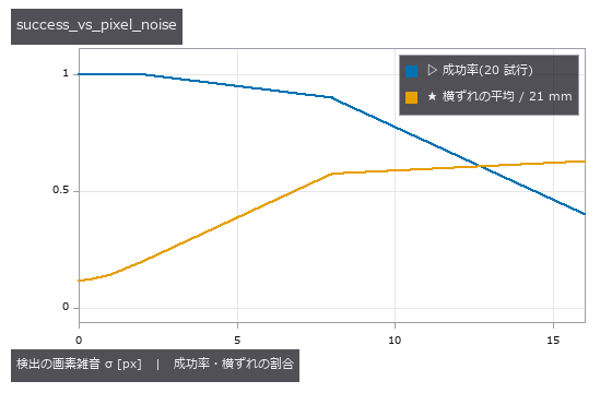
↑ Pixel noise and success rate (20 trials each). Flat up to 2 px because of the room on the cup rim.
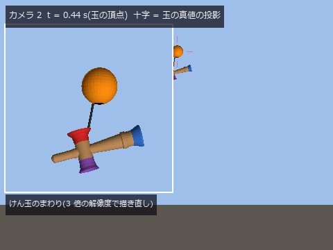
↑ A frame from camera 2 (ball at its apex). The inset re-renders the same camera at three times the resolution.
Part 3: Filming a spinning ball and reading its spin two ways — from the curve and from the markings
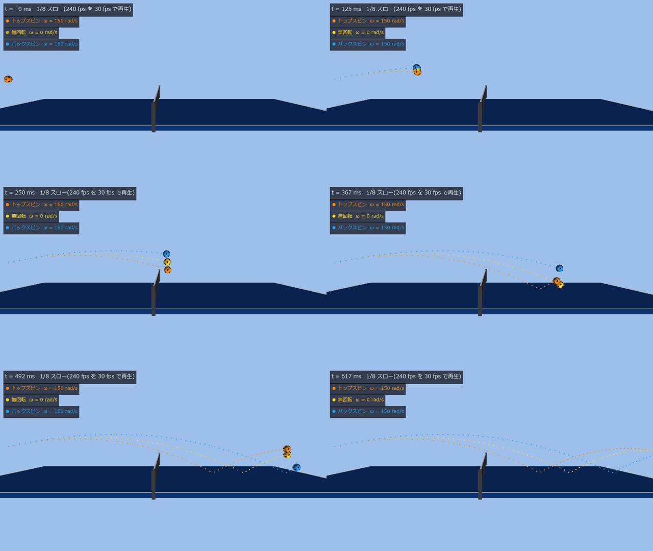
↑ Three balls launched at the same speed and angle (v₀ = (6.0, 0, 1.3) m/s), seen from the side. Topspin (orange) dips and lands short, no spin (yellow) lands in the middle, backspin (blue) floats and lands long. Only the spin (150 rad/s ≈ 1,430 rpm) differs. The balls are drawn 1.6× larger for visibility. All 240 fps frames (1/8 slow motion): MP4.
A spinning ball feels a force perpendicular to both its direction of travel and its spin axis (the Magnus force, along ω × v): downward for topspin, upward for backspin, sideways for sidespin. So the curve of the track carries the spin. The markings on the ball, on the other hand, show the rotation directly. This part reads the spin of the same serve from these two independent cues and checks one against the other.
Steps
- Film four serves that differ only in spin (top, none, back, side) with two cameras on either side of the table (240 fps, 1024 × 800).
- Find the ball by colour, triangulate, and get a 3-D track. Like a high-speed camera’s ROI readout, only a 160 × 160 px window around the constant-velocity prediction from the previous two frames is read (the full frame when the ball is lost).
- From the curve: fit the drag + Magnus equation of motion to the pre-bounce track with 9 parameters — position, velocity and spin (
fit_spin). - From the markings: film the same serve with a close-up camera (1000 fps, 20 frames) and fit the motion of the 14 black marks with Kabsch (
spin_from_markers). - Compare the two, predict the landing point from the read spin, and check it against the truth.
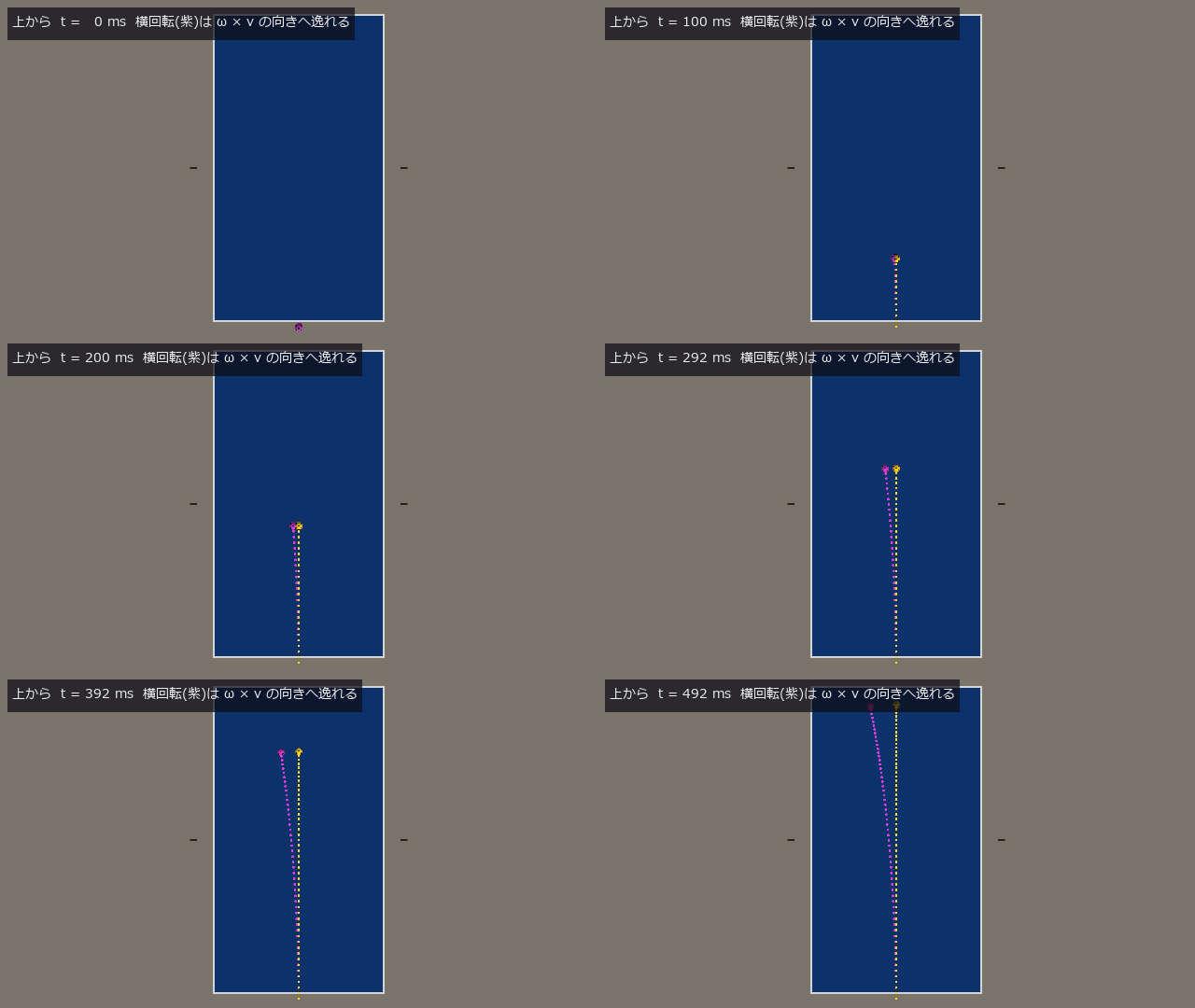
↑ From above. Sidespin (purple) leaves the same launch as no spin (yellow) and lands 15 cm to the side. MP4
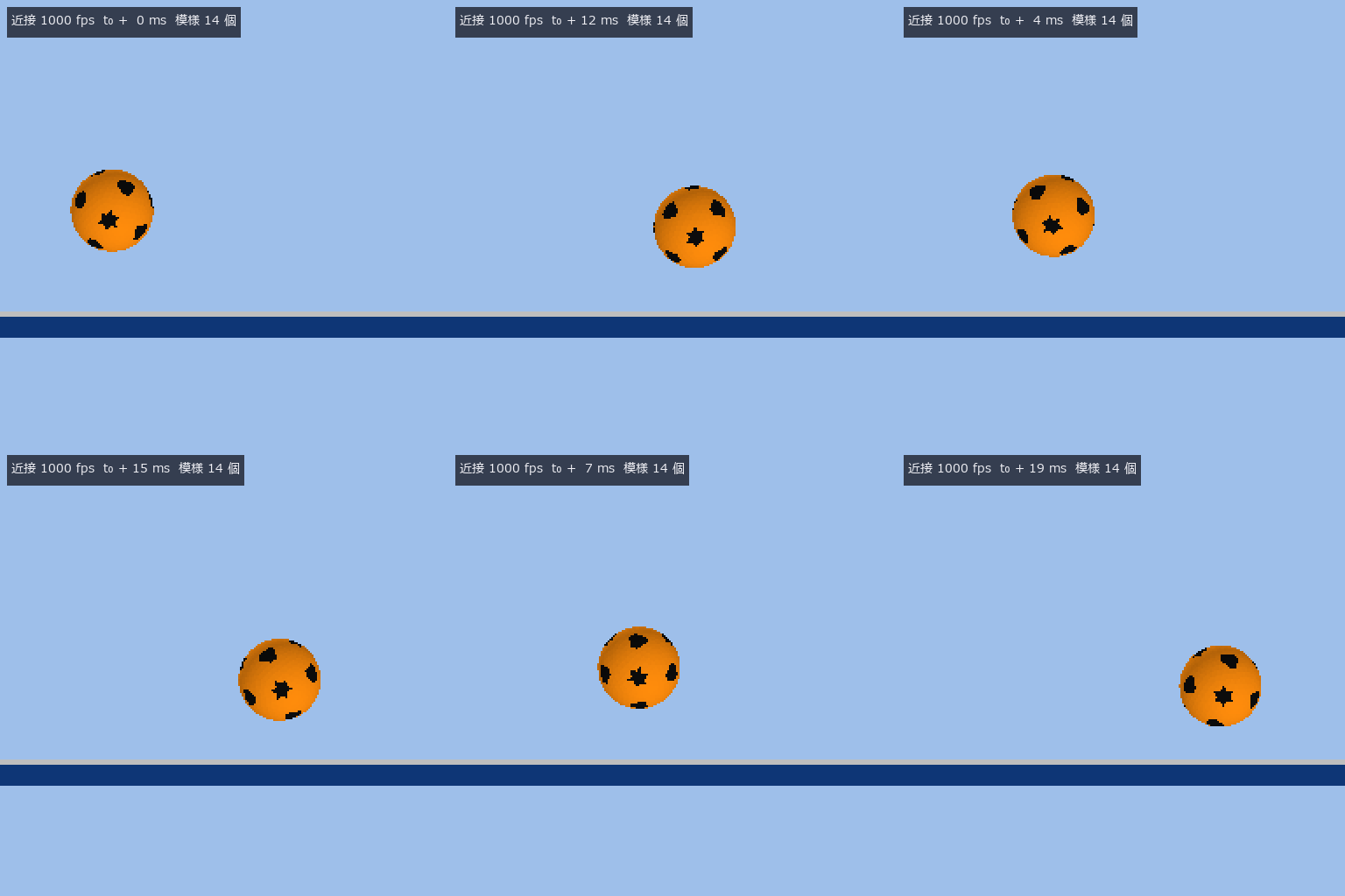
↑ Topspin seen by the close-up camera (1000 fps), 20 ms at 1/100 speed. The 4–6 visible marks are matched to the previous frame by direction and the rotation is fitted. MP4
Gates and results
| Gate | Source of truth | Result |
|---|---|---|
| Identity | feed the true track to fit_spin |
spin returned to 1.3 × 10⁻⁴ rad/s |
| Unreadable component | theorem: force is ω × v, so spin parallel to travel produces none | instantaneous acceleration differs by 4.8 × 10⁻¹⁷ m/s²; after 0.25 s the track moves 7.1 mm (5.4 cm for perpendicular spin) |
| Landing point | a world that holds the truth | landing predicted from the read spin within 2 cm for all four (x = 0.488 / 0.754 / 1.124 m; top < none < back) |
| Spin from the curve | same | perpendicular-spin error 3.9 % (top), 0.9 % (back), 1.7 % (side); 7.6 rad/s for no spin |
| Spin from the markings | same | 4.8 %, 3.2 %, 0.9 %; 2.0 rad/s for no spin |
| The two agree | second implementation (one sees only the track, the other only the marks) | 3.0 %, 3.1 %, 1.9 % |
| Track length | same | 400 % from 42 ms of track, 4 % from 321 ms |
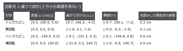
↑ The two readings side by side. The curve cannot see the component parallel to travel, so they are compared on the perpendicular component.
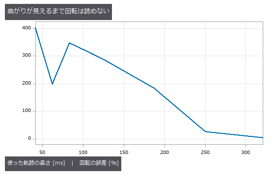
↑ Spin cannot be read until the curve shows. Using only the first n frames, the Magnus bend is buried in the 1–2 mm triangulation error while the track is short.
Pitfalls
- Spin about the direction of travel cannot be read from the curve. The Magnus force is ω × v, so the part of ω parallel to v produces no force. Most of the 22 rad/s the fit reported for the no-spin ball lies along that direction.
fit_spinreturns the readable part separately asomega_perp. The markings show every component, which is how the two cues divide the work. -
The size of the spin can be undetermined. The lift model C_L = 1/(2 + 1/S) (S = rω/v) levels off at 0.5 for large spin. With a short, noisy track the fit asks for “more force” and grows ω without bound (an undamped Gauss–Newton jumps to 10⁷ rad/s in one step). fit_spinfits with damping and returnsat_bound = Truewhen it hits the cap (1,000 rad/s by default) — do not trust the magnitude then. - The net hides half the ball. From the server-side camera, the net’s white band hides the top half of a low ball beyond the net. The colour centroid shifts to the visible lower half, up to 26 mm after triangulation. Detections whose image radius is under 0.8× their neighbours’ are dropped.
- For a ball crossing the frame, the change of line of sight looks like spin. Treating the ball’s image as a disc and turning a mark’s offset from the centre into a direction is only right when the ball is on the optical axis. A ball crossing 0.6 m away at 6 m/s turns the line of sight by 0.01 rad per ms, adding 7 % to one frame’s rotation (0.15 rad). Pass the camera K as
marker_direction(..., K)and it solves the perspective exactly by intersecting the mark’s pixel ray with the sphere.
Not suited for
- The aerodynamic model (C_d = 0.4, spin-ratio C_L) is the same one that produced the truth; reading spin from the curve assumes the model is right. Measured C_L has been reported to dip near a spin ratio of 0.5 (Miyazaki et al. 2017), so on real balls C_L has to be measured first.
- Spin is constant in flight (no decay).
- Ball detection runs on synthetic video with a known colour; there is no real lighting, blur or background. The close-up camera is conveniently placed for the 20 ms the ball is in view.
Run it
import numpy as np
import fullseye as fs

bp = fs.ledger.ball_params()                               # 40 mm, 2.7 g, drag 0.4, lift from the spin ratio
t = np.arange(0.0, 0.30, 1 / 240)                          # 0.3 s at 240 fps
f = fs.ledger.flight_ode([-1.3, 0.0, 1.01], [6.0, 0.0, 1.3], [0.0, 150.0, 0.0], bp, 0.31, 1e-4)
p = np.column_stack([np.interp(t, f["t"], f["p"][:, k]) for k in range(3)])
p_obs = p + np.random.default_rng(0).normal(0.0, 1.5e-3, p.shape)     # about 1.5 mm triangulation error

r = fs.ledger.fit_spin(t, p_obs, bp)
print(np.round(r["omega"], 1), np.round(r["omega_perp"], 1), r["at_bound"])
# [ 16.5 157.8  -5.1] [  1.5 157.7  -8.4] False      ← spin [rad/s], readable part, hit the cap?

r10 = fs.ledger.fit_spin(t[:15], p_obs[:15], bp)          # only the first 62 ms
print(np.round(r10["omega_perp"], 1), r10["at_bound"])
# [ -1.8 -93.8   8.1] True                            ← too short to read (stuck at the cap)
The whole PoC: py -3.11 examples/poc_table_tennis_spin.py (figures and videos when FULLSEYE_FIGURE_DIR is set).
Part 4: Filming a bouncing ball with a high-speed camera and reading restitution and friction — checked against published values
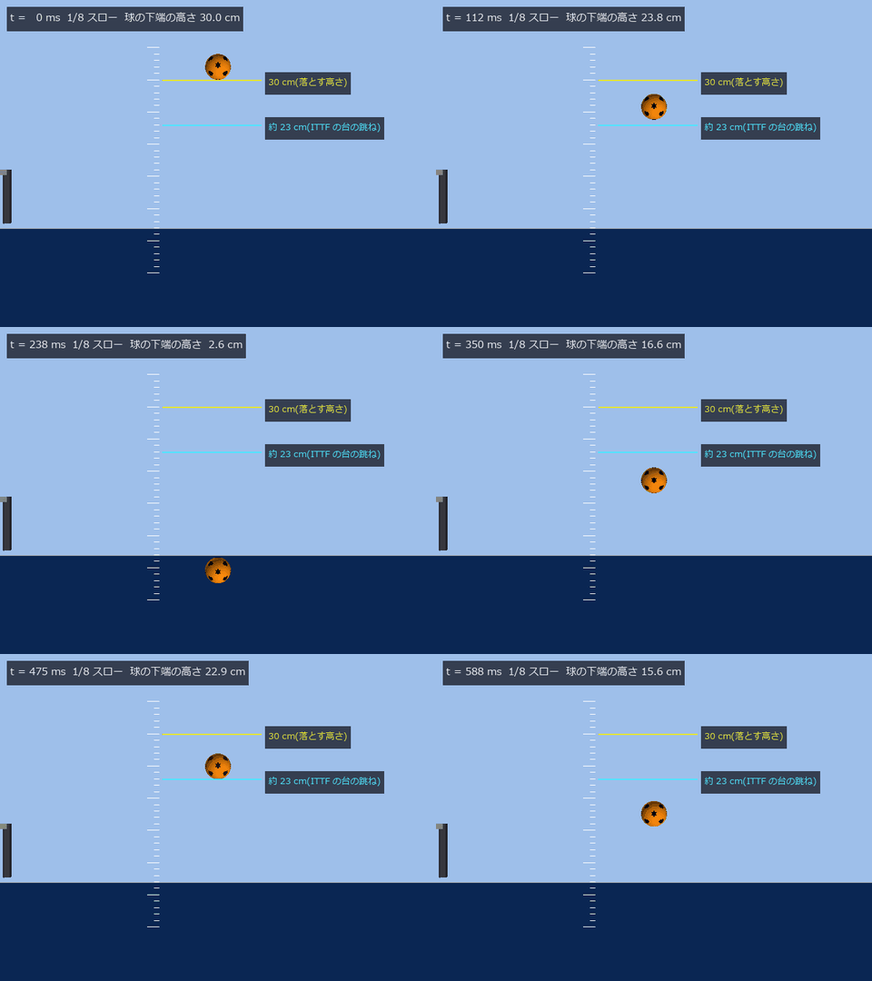
↑ The table-bounce test in the ITTF Laws (2.1.3): a ball dropped from 30 cm should bounce about 23 cm. The bounce height read from the video is 23.0 cm. The ruler is marked in 1 cm steps. All 240 fps frames (1/8 slow motion): MP4.
When a table-tennis ball bounces on the table, the coefficient of restitution e decides how much of the vertical speed survives. Friction trades horizontal speed against spin. If the contact point (where the ball touches the table) slides only a little, the sliding stops during the bounce and the ball leaves rolling; if it slides a lot, the ball leaves still sliding. Which one happens changes where the ball goes next.
This part films 22 bounces with one high-speed camera (1000 fps, from the side), reads e, the friction coefficient μ and the kind of bounce from the images alone, and checks them against published values.
Steps
- The ball’s plane of motion (the vertical plane y = 0) is known, so one camera gives positions: intersect the line of sight through the ball’s centre pixel with that plane (
ray_plane_range). - Fit the drag + Magnus equation of motion before and after the bounce and get the velocities at the moment of contact (
flight_fit). Spin comes from the ball’s marks (spin_from_marker_sequence). -
e = −v_z’/v_z. Compare the contact point’s slip s = v_x − rω before and after; for bounces that leave sliding, μ = Δv_x /((1+e) v_z ) (the formula used by Inaba et al.). - Check the kind of bounce read from the video against the closed-form boundary drawn with the measured e and μ.
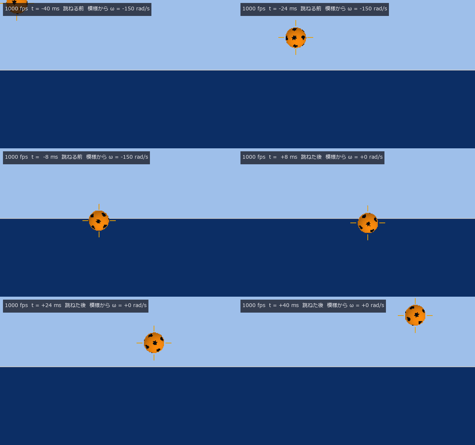
↑ A backspin bounce (−150 rad/s) at 1000 fps (1/40 speed). The contact point keeps sliding and friction almost cancels the spin (spin read from the marks: −150 → 0 rad/s). MP4
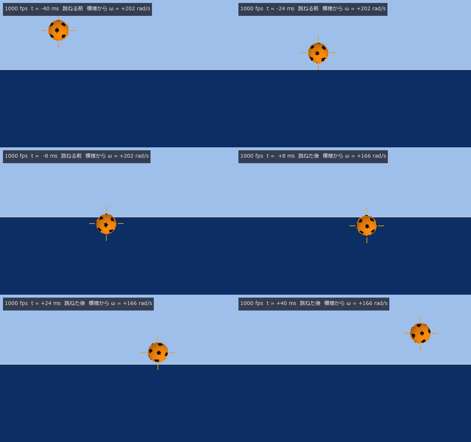
↑ A topspin bounce (+200 rad/s). The contact point slides only a little, so the sliding stops during the bounce and the ball leaves rolling (after the bounce rω’ = 3.320 m/s and v_x’ = 3.312 m/s are almost equal). MP4
Gates and results
| Gate | Source of truth | Result |
|---|---|---|
| Closed forms of the bounce | Cross 2002 (thin-shelled ball I = (2/3) m r²): a bounce that ends rolling has v_x’ = 0.6 v_x + 0.4 rω; one that keeps sliding has Δv_t = μ(1+e)|v_z|; the boundary is (2/5)|s| = μ(1+e)|v_z| | against the impulse implementation, 300 random impacts: kind 300/300, velocity difference 2.7 × 10⁻¹⁵ m/s |
| ITTF table bounce | published (Laws 2.1.3: 30 cm → about 23 cm) | 23.0 cm from the video |
| e versus impact speed | published (Inaba et al. 2017, plastic ball: −0.0058 per km/h) | slope over 22 bounces (5.0–16.4 km/h) −0.00572, 1.4 % off; median per-bounce e error 0.0004 |
| Friction coefficient | a world that holds the truth (0.25, matched to the 0.2526 intercept of Inaba et al.) | 0.250 from the 3 clearly sliding bounces |
| Kind of bounce | closed-form boundary drawn with the measured e and μ | 15 / 15 agree (1 bounce within ±10 % of the boundary is not judged) |
| Rolling | a bounce that ends rolling has rω’ = v_x’ | 0.1–2.3 % over 10 bounces |
| Zero point | a table without friction | horizontal speed changes by 0.002 m/s, spin by 0.2 % |
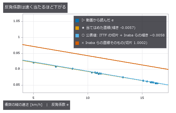
↑ The e read from the video drops as the impact gets faster; the slope agrees with Inaba et al. 2017 to 1.4 %. The upper line is their formula itself (intercept 1.0002), which sits on the livelier side of the ITTF table.
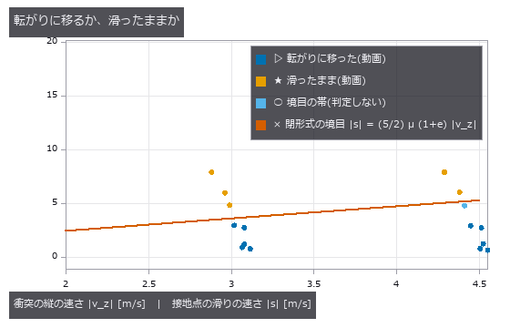
↑ Bounces below the boundary stop sliding and leave rolling; those above leave still sliding. The boundary is drawn with the μ and e read from the video.
Pitfalls
- Reading 30 cm → 23 cm as e = √(23/30) = 0.876 drops the air drag. For a 40 mm, 2.7 g ball, drag on the way down and up takes 1.3 cm, so a table with e = 0.876 bounces only 21.7 cm. The e that gives about 23 cm with drag is 0.902.
- Published values can disagree. The formula of Inaba et al. itself (e = 1.0002 − 0.0058 v) makes a table that bounces 25.5 cm from 30 cm, which does not match the ITTF’s about 23 cm. Whether this is their lab table versus the standard, or the way it was measured, has not been checked. This PoC’s table uses the ITTF value as the intercept and the slope of Inaba et al. for the speed dependence.
- A bounce that ends rolling only gives a lower bound on μ. Once the sliding stops, friction uses less impulse than μ J_n. The apparent μ of such bounces (0.03–0.24) is not μ. Measure μ only on bounces that are still sliding afterwards.
- One camera needs a known plane of motion. Here the ball is played in the vertical plane y = 0. A ball flying at an angle needs two cameras (the triangulation of Part 1).
Not suited for
- The friction coefficient is a constant. Inaba et al. measured it rising to 0.27–0.44 with the contact-point speed.
- The ball does not deform. A thin shell is reported to start buckling around 5.5 m/s, lowering e further (Rémond et al. 2022); vertical speeds here stay under 4.5 m/s.
- Synthetic video: no real lighting, blur or background.
Run it
import numpy as np
import fullseye as fs

bp = fs.ledger.ball_params()
ip = fs.ledger.impact_params(0.90, 0.25)                  # e, μ
r = bp["radius"]
v_in, n = [3.0, 0.0, -3.0], [0.0, 0.0, 1.0]

# a bounce that keeps sliding (backspin) and one that ends rolling (topspin)
for w in (-150.0, 200.0):
    b = fs.ledger.bounce(v_in, [0.0, w, 0.0], n, bp, ip)
    print(b["regime"], np.round(b["v"], 3), round(r * b["omega"][1], 3))
# slip [1.575 0.    2.7  ] -0.862        ← keeps sliding: Δv_x = μ(1+e)|v_z| = 1.425
# grip [3.4 0.  2.7] 3.4                 ← ends rolling: v_x' = 0.6·3 + 0.4·(0.02·200) = 3.4, rω' = v_x'

# recover e and μ from (v, ω) before and after (for a rolling bounce μ is only a lower bound)
b = fs.ledger.bounce(v_in, [0.0, -150.0, 0.0], n, bp, ip)
f = fs.ledger.fit_bounce(v_in, [0.0, -150.0, 0.0], b["v"], b["omega"], n, bp)
print(round(f["e"], 4), round(f["mu"], 4), f["regime"], f["mu_is_lower_bound"])
# 0.9 0.25 slip False                   ← e, μ, kind, is μ a lower bound
The whole PoC: py -3.11 examples/poc_table_tennis_bounce.py (figures and videos when FULLSEYE_FIGURE_DIR is set).
Part 5: Reading errors end the rally — how much noise and latency move the landing point, in closed form before the shot
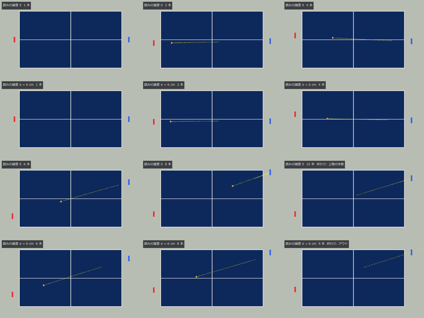
↑ Rallies seen from above (half speed). Top: no noise in the ball-position reading, the cap of 10 shots. Bottom: σ = 6 cm noise on every frame’s reading, 9 shots, ending with an out. The rackets reach the ball — the rally breaks not on a miss but on a shot aimed from a misread position that lands out. MP4
Part 1 only counted how long the rally lasted. This part works out why it breaks, as numbers, before the shot is played.
A table-tennis robot reads where the ball is, then computes a return that lands on a chosen point of the opponent’s half. If the reading is off by δ, the shot is computed from the misread position but the ball leaves from the true one. The landing point moves, and once it moves past the margin to the table edge the ball is out.
The key is how a reading error turns into a landing error: the Jacobian J, a 2 × 3 matrix. With it, the spread under noise, the probability of an out and the effect of latency can all be predicted before the shot.
In a vacuum it is a closed form
Without air, a reading error δ = (δ_x, δ_y, δ_z) moves the landing point by
| ΔL_xy = −δ_xy − (v_xy / | v_z(T) | ) δ_z |
where v_z(T) is the vertical speed on landing. Errors along and across the table come straight back with the opposite sign. A height error is stretched along the table by the landing angle. This shot lands at a shallow angle, so misreading the height by 1 cm moves the landing point 2.1 cm along the table.
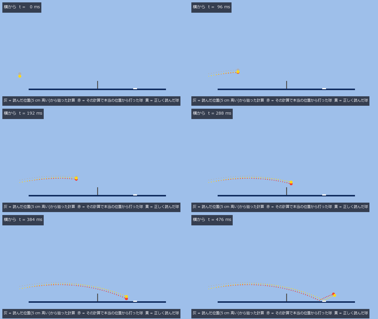
↑ From the side. Reading the ball 5 cm too high, the aim (grey) picks a lower arc, and the ball hit from its true position (red) lands 10.2 cm short. Yellow = the correctly read ball. MP4
Steps
- Through aiming, racket planning, impact and flight, nudge the reading one axis at a time and take the numerical J from how the landing point moves.
- With the air removed, check that the numerical J matches the closed form.
- With drag and Magnus, predict the landing covariance J Σ Jᵀ from the reading-noise covariance Σ, and check it against 300 shots.
- The probability of an out is the mass of that Gaussian outside the opponent’s half.
- Latency τ means a reading τ old, so the reading error is −vτ − ½gτ² ẑ; J times that is the landing error.
- Two rackets rally with noise on every frame’s reading, to see where the rally breaks.
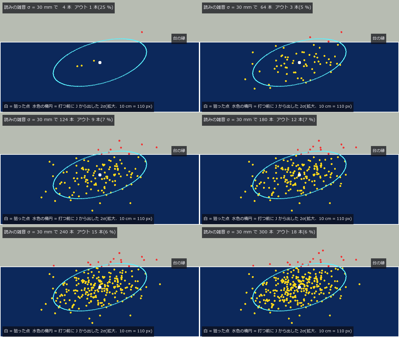
↑ Aiming 6 cm inside the table edge (white) with σ = 3 cm noise on the position reading, 300 shots. Yellow = in, red = out (6 %). The cyan ellipse is the 2σ predicted from J before any shot, long along the table — height errors are stretched that way. MP4
Gates and results
| Gate | Source of truth | Result |
|---|---|---|
| Vacuum closed form | ΔL_xy = −δ_xy − (v_xy/|v_z(T)|) δ_z | differs from the numerical J through aiming, planning, impact and flight by 2.5e-06 |
| First-order propagation | J Σ Jᵀ (with drag and Magnus) | σ = 2 cm, 300 shots: landing spread (along 4.6, across 2.0) cm, within 1.0・0.8 % of the prediction |
| Probability of an out | mass of the J Σ Jᵀ Gaussian outside the half | 6 cm from the edge with σ = 3 cm: predicted 0.043, 300 shots give 0.060 (1.5 σ binomial) |
| Latency | J · (−vτ − ½gτ² ẑ) | τ = 5 / 10 / 20 ms, off by 0.2〜0.6 % |
| Closed loop | noise-free rallies reach the cap / beyond the noise bound σ* from the margin the rally breaks | no noise: 10 shots all 4 times. σ = 6 cm (1.2 × σ* = 5.2 cm): 9・8・2・7 shots, all ending out |
| Zero point | no error lands on the target | 0.52 mm |
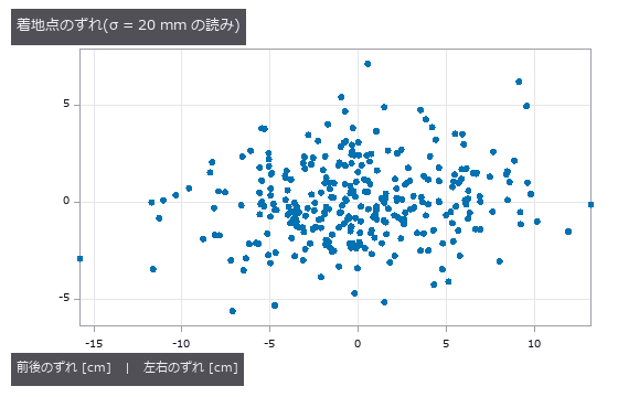
↑ Landing points of 300 shots with σ = 2 cm readings. The noise is the same size in all three directions, yet the spread is 2.2 × longer along the table.
Pitfalls
- The sign of an “old reading”. τ earlier the ball was higher and falling more slowly; with constant acceleration z(t − τ) = z − v_z τ − ½gτ². I first wrote + ½gτ². The gate compares “the landing error when actually shooting from the old reading” with “J times the same reading error”, so a wrong reading error enters both sides and still passes. A numerical integral caught it (the height error at τ = 20 ms is 0.8 cm, not 1.2 cm).
- I nearly wrote “the linearisation underestimates the tails”, and withdrew it. The first gate aimed 12 cm from the edge with σ = 5 cm: predicted 0.017, 300 shots gave 0.037 (2.7 σ binomial). With other random numbers it became 0.017 against 0.003 (1.8 σ) — the direction flipped. 300 shots cannot tell which way the approximation errs. The gate sits where the linearisation holds (6 cm from the edge, σ = 3 cm); the large-noise case is reported as numbers only.
- A video made at the rally’s time step has over 20,000 frames. Flight is integrated at 0.2 ms. The first version drew a frame every two simulation steps and the figure run was stopped for low memory. Frames are now cut by simulated time (every 0.02 s) and kept as uint8.
Not suited for
- Only the ball position is misread (velocity and spin are true). The noise is independent Gaussian per frame; systematic camera errors (calibration drift) are not included.
- The racket reproduces the planned face angle and speed exactly (no control error).
- An out is judged only by the margin to the table edge; the net is ignored (the targets are deep).
Run it
import numpy as np
import fullseye as fs

tp, rp = fs.ledger.table_params(), fs.ledger.racket_params()
bp = fs.ledger.ball_params(rho=0.0)                        # no air (to compare with the closed form)
ip = fs.ledger.impact_params(0.9, 0.25)
H = tp["height"]
p, v_in, w_in = np.array([-1.55, 0.1, H + 0.25]), np.array([-4.0, 0.2, -0.5]), np.array([0.0, -50.0, 0.0])
target, T = np.array([0.75, 0.3, H + 0.02]), 0.42


def landing(delta):
    """Landing point of a ball aimed from the misread position p + δ but hit from the true p."""
    w = np.zeros(3)
    for _ in range(3):                                     # iterate the aim with the spin after the hit
        aim = fs.ledger.aim_velocity(p + delta, target, T, bp, w)
        plan = fs.ledger.racket_plan(v_in, w_in, aim["v"], bp, rp)
        w = plan["omega_out"]
    b = fs.ledger.racket_impact(v_in, w_in, plan["normal"], plan["v_racket"], bp, rp)
    s = fs.ledger.flight_simulate(p, b["v"], b["omega"], bp, ip, 1.2, 2e-4, table_z=H)
    return s["contacts"][0]["p"][:2], b["v"]


L0, v = landing(np.zeros(3))
h = 1e-3
J = np.column_stack([(landing(h * e)[0] - landing(-h * e)[0]) / (2 * h) for e in np.eye(3)])
vz_T = v[2] - 9.81 * T
print(np.round(J, 3))
# [[-1.     0.    -2.1  ]
#  [-0.    -1.    -0.183]]
print(np.round([-v[0] / abs(vz_T), -v[1] / abs(vz_T)], 3))   # closed form, third column: −v_xy / |v_z(T)|
# [-2.1   -0.183]
The whole PoC: py -3.11 examples/poc_table_tennis_rally_loop.py (figures and videos when FULLSEYE_FIGURE_DIR is set).
Next time
The spike trick. Putting the spike into the ball’s hole. Part 2’s kendama stopped at landing the ball on a cup. Next, the hole’s direction and the ball’s spin are read from images, the condition for the spike to enter (the clearance between the hole’s rim and the tip) is written in closed form, and the spike is guided in by the image prediction.