fullseye
A Good Fit Is Not a Right Answer: Calibrating Physics-Model Coefficients to Real Images, Starting from Multivariate Analysis
日本語版: 実写に合わせて物理モデルの係数を決める
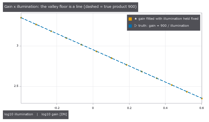
Hold the illumination at a fixed value, refit only the camera gain, and every result (orange) lands on the truth line gain x illumination = 900 (dashed). The image is explained equally well at every point, so the image alone cannot tell you which one is right.
What this is about
When a simulated image doesn’t match a photograph, the natural move is to tune the model’s coefficients - focal length, refractive index, film thickness, camera gain - until it does. This series started from two lines the author wrote down:
Given a real image, it would be nice to feed the error back and adjust the coefficients the simulation uses automatically.
Shouldn’t that start from something like multivariate analysis?
The first line is ordinary least-squares fitting. The second one is the point: unless you first find out which coefficients the photograph can actually pin down, you have no reason to trust what the fit gives you. This article shows why, with three concrete cases.
The short version:
- A small fit residual does not mean the coefficients are right. Some combinations of coefficients cannot be separated by the images (they are confounded), and when the model is missing something, the coefficients bend to absorb it and the fit still looks good.
- Multivariate analysis catches this before fitting: how to choose the capture conditions (design of experiments), which coefficients actually move the image (sensitivity), and which ones move it the same way (confounding).
- Identifiability, held-out images, residual PCA, and an absolute chi-squared test against the noise model catch it after fitting.
Every example runs from tours in Fullseye, an open-source image-measurement library (https://github.com/furuse-kazufumi/fullseye). The numbers below were checked against the printout of:
py -3.11 examples/simcal_tour.py
py -3.11 examples/simcal_checks_tour.py
Terms
| Term | In plain words | Used here for |
|---|---|---|
| knob | a model coefficient you adjust to match the images | illumination, gain, refractive index n, thickness d, focal length f |
| reduced chi^2 | residuals divided by the noise level, squared and averaged | 1 means “the residual is just noise”; 60 means 60 times the noise |
| confounding | two knobs move the image in the same way | only a combination (e.g. a product) is determined, not each knob |
| identifiability | whether the images pin a knob to a single value | if not, the fit refuses to return a value |
| holdout | images kept aside and not used for fitting | checks that the fitted model also explains images it hasn’t seen |
| residual PCA | splitting the residual images into principal components | a shape above the noise means the model is missing something |
Case 1: gain x illumination - only the product is determined
In plain words
Two knobs make the image brighter: the light level and the camera gain. Double the light and halve the gain, and the image is identical. The images determine the product illumination x gain, and nothing else.
Obvious - yet hand both knobs to a least-squares solver and it will usually return some pair of values. That pair depends on where the solver started and has nothing to do with the truth.
Figure and numbers
The opening figure fixes the illumination at 13 values from 0.4 to 4 and refits the gain each time. The truth is illumination 1.5, gain 600 (product 900). Every refitted gain lies on gain = 900 / illumination.
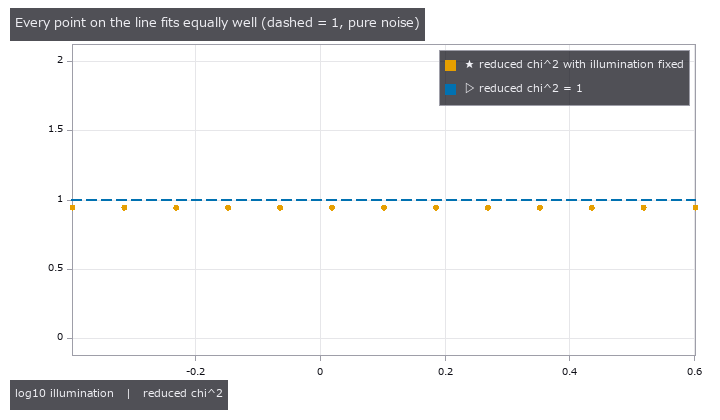
The next figure shows how well each of those fits explains the images. Every point sits at a reduced chi^2 of about 0.94, just under the pure-noise value of 1. Illumination 0.4 or 4 - the images can’t tell the difference.
Fullseye’s fitter (simcal_fit) refuses to return values in this situation and reports only what is determined:
- determined combination:
illum^1 * gain^1 = 899.4(truth 900, off by 0.06 %) - illumination and gain separately: no values (an empty dict)
- with illumination fixed at 1.5: gain = 599.6 (truth 600)
When a knob is not determined, either fix one of them from an independent source (a light meter, a datasheet value) or change the capture so that the knob does move the image. A thin film measured at a single wavelength behaves the same way: refractive index n and thickness d are not separable, and only roughly n·d (the optical path) is determined.
Case 2: a fit stuck at the wrong interference order passes every relative check
In plain words
A transparent film (n = 1.46, d = 520 nm) sits on silicon, and we measure its reflectance at 31 wavelengths from 400 to 700 nm. Reflectance oscillates with wavelength, and the number of peaks depends on the thickness. The chi^2 surface has a separate valley for each interference order, and a solver that starts in the wrong place can settle in a neighbouring one.
The fit in that neighbouring valley still looks reasonable. The trouble is that most of the usual validation checks are relative comparisons.
Figure and numbers
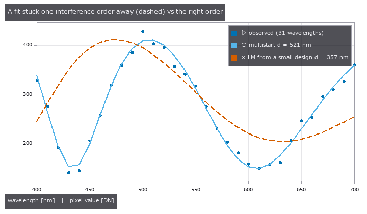
Levenberg-Marquardt started from a small design (two start points) landed at n = 1.329, d = 356.5 nm (dashed), with a reduced chi^2 of 60.4. A multistart with 16 start points reached n = 1.4591, d = 520.7 nm, reduced chi^2 0.93 (solid).
Both results were then put through the six gates of simcal_validate, using held-out images:
| Gate | Compared against | Wrong order | Right order |
|---|---|---|---|
| 1. better than the start point | chi^2 before fitting | pass | pass |
| 2. holdout / train <= 1 + tau | error ratio, held-out vs training images | pass | pass |
| 3. better than gain + offset only | the simplest possible model | pass | pass |
| 4. bounds, priors, edges | is a value pinned to the edge of its range? | pass | pass |
| 5. knobs <= image directions | over-fitting | pass | pass |
| 6. absolute: chi^2 tail probability p >= 0.001 | the noise model | fail | pass |
The wrong-order fit beats its start point, does just as well on the held-out images as on the training ones (holdout reduced chi^2 53.1, lower than the training 60.4), and beats the trivial model. Gates 1-5 all ask “is it better than something?”, so it passes all five.
Only gate 6 asks “how many times the noise is the residual?”. A reduced chi^2 of 60.4 on training and 53.1 on holdout has essentially zero probability under the noise model (p < 0.001), and that is where the fit is finally rejected.
This gate has a blind spot of its own. If the noise is overestimated (say the variance is set 4 times too large), p sticks at 1 and the gate passes; the only symptom is a reduced chi^2 well below 1. The noise model has to come from a measurement of the camera (a linear camera model in the style of EMVA 1288).
Case 3: out-of-family data shows up as a shape in residual PCA
In plain words
A model’s family is the set of images it can produce for any knob setting. Vignetting from a lens whose optical axis is off-centre cannot be produced by a centred cos⁴ model, whatever the knobs. That data is out of family.
The fit still returns numbers. Some knob absorbs what the model is missing and settles at a distorted value.
Figure and numbers
A flat target was captured at four exposure levels through a lens with its axis shifted by (5, −4) px, then fitted with the centred cos⁴ model (knobs: focal length f, gain, black level):
- f = 41.75 px (truth 40): a value comes back, 4 % off
- reduced chi^2 = 31.6
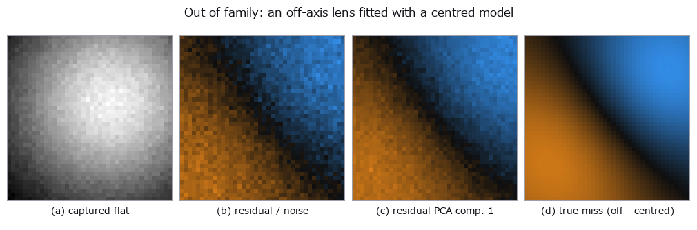
From left: the captured flat, the residual divided by the noise, the first principal component of the four residual images, and the true miss (off-axis image minus the centred model). The first component matches the true miss with a correlation of 0.99.
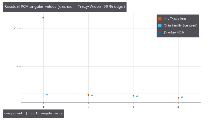
For pure noise, the singular values stay below an edge set by random-matrix theory (the 99 % point of the Tracy-Widom distribution, 42.6 here). With the off-axis lens the first singular value is 444, more than ten times the edge. With a centred lens (in family) all four stay below it. simcal_discrepancy then notes “one component of structure above the noise; the uncertainties are optimistic”.
Residual PCA tells you the shape of what is missing. Here, one look at the first component says “the vignetting centre has moved”, which is what tells you whether to add an optical-axis knob to the model.
How to use it
- Before fitting, measure each knob’s sensitivity (
simcal_screen, a Morris screen) to find knobs that do nothing and pairs that are confounded. - If a combination is not determined, change the capture (more wavelengths, a test chart) or fix one knob from an independent value.
- Fit (
simcal_fit). Use multistart when the problem has several valleys. - Run the six gates on held-out images (
simcal_validate). Keep the absolute chi^2 gate on. - Look at the shape of what is missing with residual PCA (
simcal_discrepancy).
import fullseye as fs
L = fs.ledger

obs = L.simcal_observe(model, images)          # pair the model with the images
screen = L.simcal_screen(obs)                  # moves the image / does nothing / only in combination
fit = L.simcal_fit(obs)                        # refuses if a knob is not determined
checked = L.simcal_validate(fit, holdout)      # the six gates
report = L.simcal_discrepancy(checked)         # residual PCA
print(L.simcal_report(report)["text"])
How to build model is shown at the top of examples/simcal_tour.py.
Limits
- Alignment is whole-pixel only; sub-pixel shifts stay in the residual.
- The yardstick is the camera noise model. Get the noise wrong and the bounds and intervals are wrong too.
- With several valleys and too few start points the fit can land in the wrong one. It still returns values, and says so through a warning and gate 6.
Part 2: fitting to real images, and fitting a model that is solved until it converges
What this part covers
Every example in part 1 used synthetic images. That is the right place to check that the gates ring correctly, because the truth is yours to set. With real images you choose neither the noise level nor what the model is missing. This part covers three calibrations on real images, plus one case where the observation is synthetic but the forward model is solved by iteration.
The short version:
- On real images, the gate that stopped a fit tells you more than the gates it passed. In all four cases, a model that returned numbers was stopped by the absolute chi^2 gate (or had its values withdrawn).
- A narrow interval does not mean a right answer. A normal-incidence thin-film model gave the thickness to within +-0.03 nm and missed the reference value.
- A quantity the images do not determine should come back as “not determined”. The cross-colour pixel-shift offset and the lower bound on the entrance-pupil distance are examples.
- A model fitted without deciding how many reflections to count fits with an impossible value (an albedo above 1). The count can be set from the noise level.
The numbers match both the printout of the four runs below and the numbers.json (the part2 entry) written by tools/gen_simcal_article_figs.py, which also draws the figures. Each PoC downloads its real images from the public source and caches them (only the thin-film spectrum is bundled in the repository).
py -3.11 examples/poc_simcal_thin_film.py
py -3.11 examples/poc_simcal_telecentric.py
py -3.11 examples/poc_simcal_pixel_shift.py
py -3.11 examples/poc_pocket_interreflection.py
Terms (new in this part)
| Term | In plain words | Used here for |
|---|---|---|
| profile likelihood | hold one knob fixed, refit the others, and watch how chi^2 grows | the range where the growth stays below 3.84 is the 95 % interval |
| pure error | noise estimated from disagreement between nearby points alone, without using the model | a noise yardstick that does not include what the model is missing |
| jackknife | leave out one group of data at a time, refit, and read the uncertainty from the spread of the answers | leaving out one ring at a time |
| phase correlation | reading the offset between two images from the peak of a frequency-domain correlation | a second method to check simcal against |
| interreflection | light reflected by one wall lighting another surface | nearly half the brightness of a pocket floor |
| converged solution | reflections counted until the added part is buried in the noise | matches an observation drawn with the true coefficients |
Case 4: a measured thin film - a narrow interval can still miss the reference
In plain words
There is a measured microspectroscopy reflectance spectrum of a silicon oxide film (SiO₂) on silicon, from 440 to 950 nm. The paper that published it gives a reference thickness of 98.5 nm. Following the same recipe as Case 2 in part 1, five knobs were fitted: thickness d, the dispersion of the refractive index (Cauchy A and B), the numerical aperture NA of the objective, and gain.
The noise level came from a separate measurement of bare silicon (sigma = 0.00054 in reflectance). Taking it from the residual of the very spectrum being fitted would count what the model is missing as noise.
Figure and numbers
These five knobs can cover for each other in this spectrum (local collinearity). So simcal_fit refuses to return a point estimate and answers knob by knob. Thickness d, A and gain are determined; B and NA have only an upper limit (B is at most 1977 nm²).
The profile likelihood of the thickness is the figure below. The 95 % interval is [94.6, 99.0] nm (width 4.4 nm) and contains the reference 98.5 nm. All six gates pass on 328 held-out wavelengths (absolute reduced chi^2 is 0.29 on training and 0.34 on holdout). The status is partial: B and NA have only upper limits, so not every knob gets a point estimate.
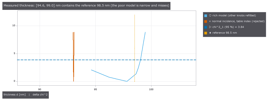
Light blue is the five-knob model. The range under the dashed 3.84 line is the 95 % interval, and the dotted reference 98.5 nm lies inside it. Orange is a poor model, “normal incidence with the index from a materials table”. Its interval, [93.02, 93.07] nm, is thin and misses the reference by about 5 nm.
A reduced chi^2 below 1 (0.29) comes from a generous noise floor. The sigma taken from the bare-silicon measurement is larger than the white part measured by second differences along the wavelength (0.00014).
The poor model explains the same spectrum well to the eye. Dividing the residual by the noise shows the difference.
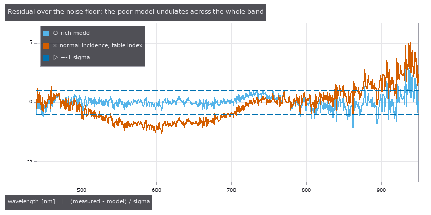
Light blue is the residual of the rich model, orange that of the normal-incidence, table-index model. Orange undulates across the whole band and leaves the +-1 sigma lines (dashed).
Here is how the poor models fared at the gates:
- normal incidence, table index: reduced chi^2 1.98. The absolute gate rejects it.
- no dispersion, constant n (the table value at 589 nm): reduced chi^2 5.57. Rejected as well.
- no dispersion, constant n, but with A and NA free: reduced chi^2 0.29, passes, interval [96.4, 99.0] nm. This one cannot be rejected. A 98 nm film has less than one fringe in the band, so dispersion is not visible.
Last, the same film calibrated on a real microscope photograph (camera model unknown, JPEG). The photograph determines only the light-source colour temperature and the vignetting; thickness, refractive index, gain and gamma are determined only in combination. Fixing the index at the table value gives a thin interval, d = 86.65 nm ([86.43, 86.86]), but it is 12 % below the reference, reduced chi^2 is 11.7, and residual PCA finds two components of structure and rejects it. The model has only the CIE 1931 colour-matching functions, not the actual camera’s spectral sensitivity, and that is the cause.
Limits
- With a thin (98 nm) film, the measurement cannot determine dispersion. A thicker film or a wider band is needed.
- For a photograph, no thickness can be reported unless the model includes the camera’s spectral sensitivity. A narrow interval does not rescue it.
Case 5: a real telecentric image - the entrance pupil is only “far”
In plain words
An object-side telecentric lens keeps the image scale unchanged when the object distance changes. For a perfectly telecentric lens the entrance pupil is at infinity. A real lens has a finite distance L to the entrance pupil, and the farther its inverse 1/L (the telecentricity) is from 0, the more it behaves like an ordinary lens.
An imaging model with eight coefficients was fitted to a real image of a plate tilted by 29.5 degrees (concentric rings 1 mm apart) taken through a telecentric lens: plate tilt, orientation, centre position, scale (px/mm), the reference ring radius, radial distortion k1 and 1/L. The observation is “the distance from the centre hole to the centre line of ring k, along a measuring line at angle a”. Of the points on the eight rings, those on the measuring lines at 0, 4, … degrees (330 points) were used for training and those at 2, 6, … degrees were held out.
Figure and numbers
First, the noise was set independently of the model. A local quadratic was fitted to the points at 4-degree steps along the measuring line, and the residual of that fit (pure error) gives sigma = 1.12 px. Fitting with this noise leaves a residual of 1.35 px and the absolute gate fails (reduced chi^2 is 1.51 on training with p = 7.5e-9, and 1.81 on holdout). simcal_validate withdraws the numbers.
The figure below divides the 47 mean residuals per ring and per 30 degrees by their standard error from the pure error. The sum of squares is 96, and under noise alone it should follow chi^2(47), whose tail probability is p = 3.2e-5. Smooth ring-by-ring disagreement remains, in a form that resembles the quirks of the plate’s printing and edge reading.
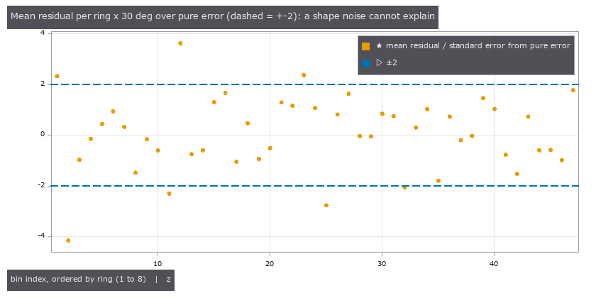
The horizontal axis numbers the 30-degree sectors, ordered by ring 1 to 8. The vertical axis is the mean residual divided by its standard error from the pure error. The dashed lines are +-2.
Residual PCA on this residual says white (no structure). In the shape of a ring x measuring-line matrix, the disagreement does not stand out as a principal component. Here the absolute gate and the per-sector means do the stopping.
Adding the disagreement as white variance (sigma = 1.37 px) and refitting passes all six gates. Before reporting numbers, though, the uncertainty was checked by a different method: a jackknife that leaves out one ring at a time. For 1/L the ratio of jackknife to Laplace approximation is 0.77, the same size.
- scale: 252.14 +- 0.18 px/mm (the paper’s values are 252.0, and a range of 251.8 to 253.0)
- 1/L = 0.50 +- 0.18 /m. The entrance pupil is farther than 1.16 m (2 sigma).
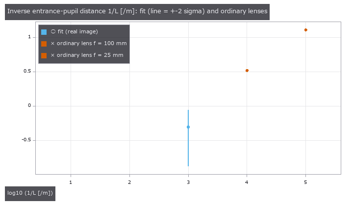
Light blue is the fitted 1/L (the line is +-2 sigma). Orange marks two ordinary lenses, focal length 100 mm (entrance pupil 302 mm) and 25 mm. The vertical axis is logarithmic.
Ordinary lenses (1/L = 3.31 /m for 100 mm, 12.9 /m for 25 mm) are ruled out by this plate. On the other hand 1/L is 2.7 sigma from 0, so the lens cannot be called perfectly telecentric either. It may be mixed with the assumption that the optical axis is at the image centre, or with the rings’ own quirks; the difference does not reach 3 sigma, so the calculation does not decide either way.
A synthetic run of the same procedure showed the following. On a plate with a smooth ring-by-ring disagreement put in, all six gates pass and yet the jackknife uncertainty is 2.4 times the Laplace one (1.0 times on a plate without disagreement). Laplace is optimistic. When disagreement is left over, passing the gates is not enough reason to trust the uncertainty.
Limits
- The observation is only the distance to the ring centre lines. The image itself is not fitted.
- The entrance pupil is “farther than 1.16 m”. No point estimate of the distance is given.
- Treating the disagreement as white variance is an approximation that holds when the ring-by-ring disagreements are independent.
Case 6: real pixel-shift frames - only what is determined can be cross-checked
In plain words
Pixel shift captures the same scene in four frames while moving the sensor, to fill the gaps between pixels and raise the resolution. The amounts moved (the offsets) are nominal values, and a real machine departs from them. These offsets are fitted from the four captured images.
The sensor has a colour-filter array (RGGB), so the same pixel sees a different colour in different frames. So pairs with a nominal diagonal offset of (+-1, +-1 pixel) are used. In such a pair green (G) overlaps G, so no colour difference enters. Only G is placed on a lattice rotated by 45 degrees, the first frame is the reference and is interpolated by a cubic spline, and the G lattice of the other frame is predicted. The lattice is cut into 16 tiles and the offset (dr, dc) is fitted tile by tile. The pairs are frame 1 to 3 and frame 2 to 4.
Figure and numbers
The noise comes from the variance of the difference of a G pair looking at the same point on bright paper (K = 0.363 DN per electron).
Both dr and dc are determined in all 32 tiles. Each tile is compared with phase correlation (read to sub-pixel precision), an independent method.
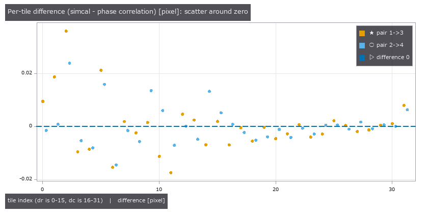
The per-tile difference (simcal minus phase correlation). The left 16 points are dr and the right 16 are dc; orange is the frame 1 to 3 pair, light blue the frame 2 to 4 pair. The dashed line is zero.
The mean of the per-tile differences is (+0.0016, -0.0011) pixel for frame 1 to 3 and (+0.0019, -0.0007) pixel for frame 2 to 4. A paired t-test gives p = 0.22 and 0.30 (the smaller of dr and dc in each pair), indistinguishable from 0. Individual tiles scatter by up to 0.036 pixel. The median reduced chi^2 is 1.55 and 1.02, not returning to 1. The noise K comes from a single point, and per-pixel sensitivity variation is not separated out.
The other pair, frame 1 to 2, is the one where G sees R and B pixels. With the same model (the whole mosaic as the reference) the reduced chi^2 is 31.1, dr sticks to the edge of its range, and simcal withdraws the value (status partial). The diagonal pair with the same model gives 1.84. On a synthetic image the same pair gets values back from the same model, so the difference is physics the model does not have.
In other words, the offset between the two pairs is not determined by this achromatic chart. Withholding a number is how the result says so.
Limits
- Only diagonal pairs where the same colour overlaps are cross-checked. Determining cross-colour offsets would take a coloured subject or a model with lateral colour.
- The phase correlation it is checked against is also an estimate, not the truth. All that can be said is that the two methods agree.
- Per-pixel sensitivity variation and dark readout noise are not in the noise model.
Case 7: a model that does not count reflections fits with an impossible value
In this case alone the observation is synthetic (no real image is used). It belongs in part 2 because it shows how the same gates behave when the forward model is solved by iteration.
In plain words
In a concave part (a machined pocket, an inside corner), light reflected by the opposite wall lights the floor (interreflection). A model that counts direct light only does not have this part. The missing brightness is absorbed by the albedo or the light intensity and plausibly fits.
Three models were fitted to a synthetic observation of a part (albedo 0.7) with a 20 x 14 mm, 10 mm deep pocket in a 28 x 22 x 14 mm block, captured with dome lighting and a linear camera. On average 48 % of the pocket floor’s brightness (up to 62 % among the pocket pixels) is interreflection.
- a model that counts direct light only
- a model that counts one bounce
- a model that counts reflections until the added part is buried in the noise (the converged solution), using progressive radiosity
There are two knobs, albedo and light intensity, with true values 0.70 and 1.00.
Figure and numbers

The direct-only model fits with albedo 1.32. An albedo above 1 means more light goes out than comes in, which is physically impossible. Its reduced chi^2 is 23.95, residual PCA finds four components of structure, and the absolute gate and the “better than gain and offset only” gate fail it. The one-bounce model gives albedo 0.873 and reduced chi^2 7.89. The converged solution returns albedo 0.6996 and light 0.9999, back to the truth, with reduced chi^2 of 1.01 on training and 1.04 on holdout, white residuals, and all six gates passed.
How many reflections are enough can also be set from the noise.
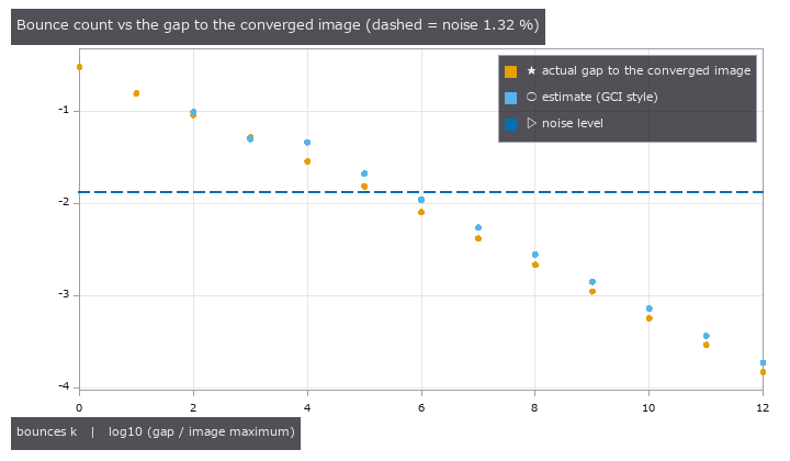
Orange is the actual gap between the image stopped after k bounces and the converged one (relative to the image maximum, logarithmic). Light blue is a GCI-style estimate from the increments of the iteration. The dashed line is the observation noise (1.32 % at the brightest pixel).
Taking the noise as the tolerance, the number of bounces needed is 7 (the actual gap then is 0.42 %). The estimate can be trusted only in the asymptotic range, from the step where the ratio between neighbouring increments has moved by less than 5 % twice in a row. Before it, at k = 3, the estimate 0.0501 fell below the actual gap 0.0523. That is an optimistic estimate, and it stays in the text.
The only link to real images is a quoted number. In Table 2 of a paper that measured three concave shapes in two materials with a time-of-flight (ToF) camera, adding one bounce brings the mean absolute error to 0.20 to 0.47 times that of direct light only. In this example’s intensity image the same ratio is 0.53 (the converged solution’s error is 22.4 DN, next to the noise-only estimate of 21.9 DN). The paper’s quantity is distance and this one is intensity, so all that is compared is the direction and size of “what direct light alone leaves out”. The paper’s values are quoted unchanged and the ratios are computed here.
Limits
- The observation is synthetic. On a real concave part the reflection properties (specular, translucent) may lie outside the model.
- Every surface is treated as diffuse (Lambertian). Specular interreflection and tilted faces are not included.
- The converged solution takes about 10 times as long as the direct-only model (32.5 s against 3.2 s in our run). The number of iterations and the patch size must be set to the noise level.
How to carry this part into your own work
- Take the noise from a measurement separate from the model (a bare substrate, a pair that sees the same point, disagreement between nearby points).
- Before fitting, separate what is determined from what is not. Answer an undetermined quantity with an interval or an upper limit.
- Keep the absolute chi^2 gate and residual PCA. A narrow interval is not a reason to pass.
- When disagreement is left over, check the uncertainty by a different method such as a jackknife before reporting a number.
- For a model solved by iteration, set the count from the noise level and look at it beside a direct-only model.
Sources (real images and quoted numbers)
- Thin-film reflectance spectrum and microscope photograph: J. Schwarz et al., “Spectro-Spatial Unmixing in Optical Microspectroscopy for Thickness Determination of Layered Materials”, Advanced Optical Materials (2024), doi:10.1002/adom.202402502. Data: doi:10.5281/zenodo.13753754. CC BY 4.0. Changes: labels re-assigned and values rounded; the photograph reduced to 640 x 360.
- Image of the telecentric plate: A. W. Stark et al., “Telecentric stereo 3D imaging with isotropic micrometer resolution bridges macro- and microscale in small Lepidopterans”, Scientific Reports 15, 28690 (2025), doi:10.1038/s41598-025-13795-6. Image: doi:10.6084/m9.figshare.c.7652423. CC BY 4.0. Changes: converted to grayscale, reduced, ring points extracted. No image is reproduced in this article.
- The four pixel-shift frames: G. Qian et al., “Rethinking Learning-based Demosaicing, Denoising, and Super-Resolution Pipeline”, ICCP 2022 (arXiv:1905.02538). CC BY 4.0. Changes: cropped, white balanced. No image is reproduced in this article.
- The quoted MAE ratios: D. Bulczak, M. Lambers, A. Kolb, “Quantified, Interactive Simulation of AMCW ToF Camera Including Multipath Effects”, Sensors 18(1):13 (2018), doi:10.3390/s18010013. CC BY 4.0. The values in Table 2 are quoted unchanged; the ratios are computed here.
CC BY 4.0: https://creativecommons.org/licenses/by/4.0/
Where the series stands
| Part | Topic | Status |
|---|---|---|
| 1 | Synthetic images: undetermined coefficients, the wrong interference order, out-of-family data | published |
| 2 | Real thin-film, telecentric and pixel-shift images, and an interreflection model solved until it converges (the Part 2 section above) | added |
| 3 | What Part 2 left open (cross-colour offsets, the telecentricity of the entrance pupil, dispersion in thin films) | planned |
Coming next
Part 2 stopped at answering “not determined” for what the images do not determine. Three points remain: the offset of the cross-colour pair in pixel shift, the 1/L of the telecentric lens being 2.7 sigma from 0, and the failure to reject a dispersion-free model on a thin film. Next time we look at which of these real data can settle.