fullseye
Language: 日本語 · English
It Passed Every Static Test, Then Failed Completely the Moment It Started Walking — Putting a Connectome-Constrained Fly Visual Model on a Body
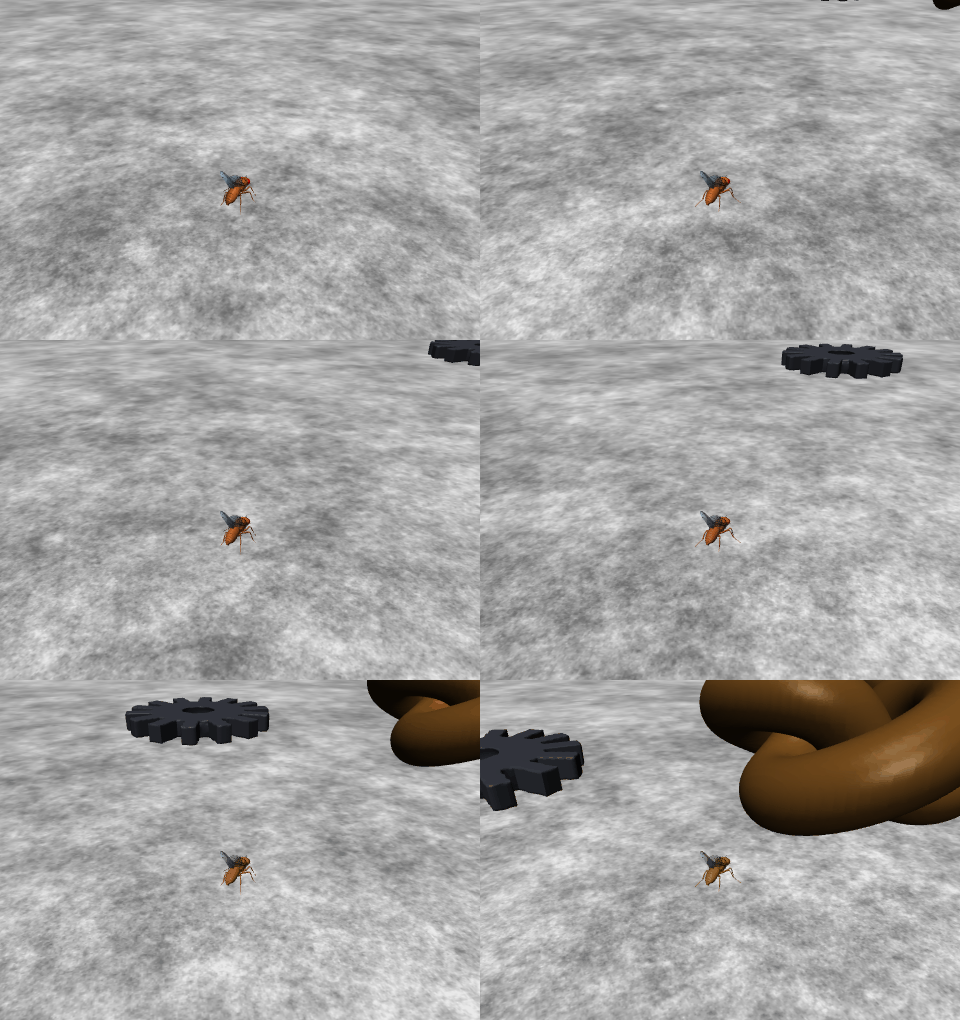
↑ The moving picture first. A physically simulated *Drosophila walks towards the brown target guided by nothing but the image on its compound eye (3× speed, external camera). The steering correction comes from an optic lobe model whose wiring is fixed by the measured connectome. The legs look like a tripod gait, but walking here is kinematic, not leg dynamics — the table below states exactly what is real and what was written by hand before any numbers appear.*
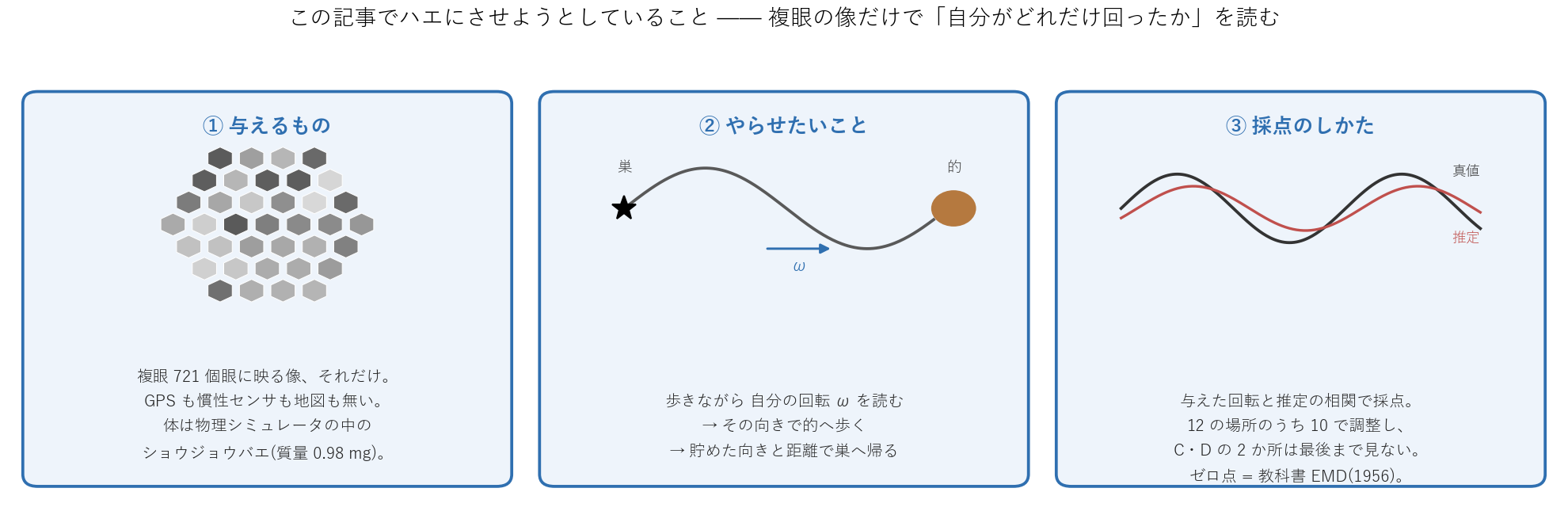
↑ The whole task in one picture. ① The input is the compound-eye image alone — no GPS, no inertial sensor, no map. ② Read your own rotation while walking, steer to the target with it, then return to the nest from the heading and distance you accumulated. ③ Scoring is the correlation against the imposed rotation, and 2 of the 12 places (C and D) are never used for selection or tuning. The null baseline is the textbook motion detector of 1956. Figure labels are in Japanese; every item is repeated in the text.
TL;DR
- A pretrained visual model of the fruit fly optic lobe — one whose wiring is fixed by the measured connectome — was mounted on a physically simulated fly body and run in closed loop: compound eye → optic lobe → steering. It passed every test built by rotating the fly in place (monotonicity, symmetry, latency), and then failed completely (correlation 0.06–0.51) when asked to read the same quantity while walking. A test built under different motion conditions than the deployment guarantees nothing.
- The cause was not the model but the world. Optic flow from translation scales as speed ÷ distance; flow from rotation does not depend on distance at all. With the eyes 1.2 mm above the floor, the floor streams past at 330–1000°/s — beyond the passband of the motion detectors, pure noise. Reading only above the horizon gives correlation 0.98. But in a world whose distant background has no texture, no motion detector can read rotation at all. Measure the stimulus statistics before you suspect the model.
- Being a good sensor is not the same as improving behaviour. Feeding that estimate into steering changed arrivals from 7/12 to 6/12 — within noise. A hand-written fixation behaviour dominated. Sensor fidelity and behavioural performance must be measured, and reported, separately.
- Evolving the free parameters showed that more degrees of freedom destroy generalisation when data is scarce. Evolving all 734 free parameters on 2 scenes pushed training to +0.76 while held-out scenes fell to −0.35 (worse than before evolution). Compressing the same search to 260 per-cell-type modulations gave +0.70. With 10 training scenes the two are nearly equal (0.916 vs 0.914). Solving the readout by ridge regression reproduced the same shape (5768 weights vs 80 weights).
- Even when behaviour improves, biological realism degrades. The solution that generalised on 10 scenes had direction selectivity in only 1 of 8 T4/T5 types, down from 3. A behavioural objective alone does not produce neural properties.
-
Driving a central-complex model (ring attractor + path integration) with the visually estimated angular velocity does get the agent home, but the dominant error term is not the gain mismatch (3.8 points) — it is the residual noise behind a correlation of 0.977 (12.4 points). No amount of careful calibration removes it.
- The eye itself is a design, too. Run the compound-eye optics (inter-ommatidial angle Δφ, acceptance angle Δρ, count) through closed-form operators and you can put a number on things like a narrow acceptance angle inventing a coarse grating that was never in the input — predicted 16.1°, measured 16.2°, and 223× smaller at the fly’s own acceptance angle. Figure and a few lines of code in section 0.
This is not an article about reproducing a fly brain. It is about where a pretrained model starts lying once you mount it in your own system — stated in numbers. The same traps appear when you put someone else’s pretrained model on your robot or your production line.
Experiments so far (this table grows)
One experiment = one question. This article is appended to every time an experiment finishes. The “current answer” column is the measurement as it stands, and it can be overturned — one entry already was, and the retraction is kept in §8.
| Question | Current answer | Section |
|---|---|---|
| Does a test built by rotating in place predict performance while walking? | No. Correlation 0.06–0.51 — a total failure | §1 |
| Does texture in the distance make rotation readable while walking? | Yes. Correlation 0.98 (0.06 without the band) | §2 |
| Does a better sensor mean better behaviour? | No change. Arrivals 7 → 6 of 12 | §3 |
| How many points of performance is the connectome wiring worth? | 0.14–0.20. Preprocessing alone takes 0.6 → 0.8 | §4 |
| Does evolving all 734 free parameters generalise? | 2 scenes overfit (−0.25); 10 scenes generalise (+0.92) | §5 |
| What if the search is compressed to 260 per-cell-type dims? | Wins on little data (+0.71), ties on plenty (+0.91) | §5 |
| What if the readout is solved by regression instead? | Same shape: 80 weights ≫ 5768 weights | §5 |
| Does better behaviour bring biological realism with it? | The opposite. Direction selectivity 3/8 → 1/8; untrained is 0/8 | §6 |
| Can the visual estimate drive central-complex homing? | Yes. The first numbers were retracted — the compass had not been calibrated (second entry in §8). Calibrated: the raw estimate homes at 2.1 %, amplitude correction makes it worse (12.4 %) | §7 → appendix |
| Does deceleration interfere with the memory update? | No. The two things that looked like interference were something else: a 10.8 % compass gain error, and an unstable equilibrium of a rule in which steering and speed both vanish with |H| | appendix |
| Does enlarging the eye break it? | No — and the first conclusion here was retracted | §8 |
| Does shuffling the wiring cost performance? | Not measurable. Two shuffles differ from each other 3× more | appendix |
| Does a staged curriculum produce direction selectivity? | Yes (0/8 → 5/8) — and the final behavioural stage destroys it (→ 1/8) | appendix |
Glossary (worth reading first)
- Connectome —— The map of which neuron connects to which, reconstructed from serial electron microscopy. For Drosophila this now exists at whole-brain scale, so “which cell type contacts which, and with how many synapses” is known.
- Connectome-constrained model —— A network whose wiring (who connects to whom, excitatory or inhibitory) is fixed from the measured connectome, leaving only continuous values (per-cell-type bias, time constant, synaptic strength) to be learned. Here: flyvis (Lappalainen et al., 2024), the optic lobe model, with 734 free parameters.
- Ommatidium —— One tube of a compound eye. Here 721 of them, 4.63° between optical axes (Δφ), 8.23° Gaussian acceptance angle (Δρ).
- T4 / T5 —— The workhorses of fly motion detection: T4 for brightening edges, T5 for darkening edges, each split into four directions (a/b/c/d).
- DSI (direction selectivity index) —— Normalised difference between the response to the preferred and the opposite direction. Here a cell type counts as selective at DSI ≥ 0.3.
- EMD (elementary motion detector) —— The textbook motion detector of Hassenstein and Reichardt (1956): take two neighbouring pixels, delay one, multiply. Used here as the null baseline.
- Self-rotation (yaw rate) —— How fast the agent is turning. Reading this from vision alone is the main task of this article.
- Hold-out —— Conditions never used for selection or tuning. Of 12 “places” (worlds with different background layouts), two (C and D) were kept unseen until the very end.
- Path integration —— Accumulating heading and speed into a running “home vector”. In insects this lives in the central complex.
- Genomic bottleneck —— The constraint that a genome cannot possibly specify every synapse, so what it can encode is closer to per-cell-type rules (Zador, 2019). This is the subject of the second half.
What is real, and where the hand-written part begins
This table comes first. Without it, a reader will assume the fly’s brain did all of it.
| Part | What it is | Origin |
|---|---|---|
| Body | Full-body Drosophila model (mass 0.98 mg, cm/g/s units) in a physics simulator | Public model (flybody) |
| Walking | Leg stance patterns are kinematic — it is not walking by leg dynamics | Hand-written |
| Eye | Three body-mounted cameras resampled onto 721 hexagonal ommatidia (including the 1.118× diagonal distortion) | Hand-written (geometry matched to the public model) |
| Optic lobe | 65 cell types, wiring fixed, 734 free parameters, pretrained | Public model (flyvis) |
| Readout | One expression: “above the horizon, (preferred − opposite) ÷ sum” | Hand-written, zero parameters |
| Behaviour | Fixate on something darker than the sky, plus optomotor feedback and efference copy | Hand-written |
| World | Floor, sky, a target, distractors. The target stands in for dung: a knot implicit surface (knot_sdf — an organic shape whose silhouette changes from every viewing angle); the distractors are a gear (gear_sdf) and a gyroid sphere (gyroid_sphere_sdf). The sky texture is synthetic |
Hand-written |
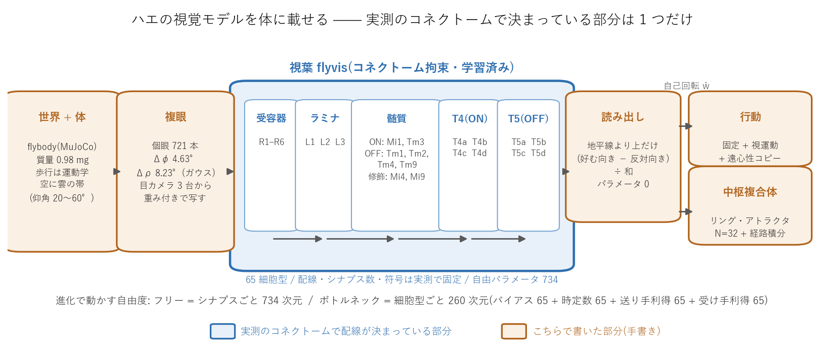
↑ The signal path and the boundary between real and hand-written. Only the blue box is wired by the measured connectome — the flyvis optic lobe, 65 cell types, in the order light travels: receptors R1–R6 → lamina L1/L2/L3 → medulla (ON: Mi1, Tm3 / OFF: Tm1, Tm2, Tm4, Tm9 / modulatory: Mi4, Mi9) → T4a–d (ON) → T5a–d (OFF). Every orange box was written here. Evolution moves only the continuous values inside the blue box; not one new connection is ever added. Figure labels are in Japanese; the same content is in the table above.
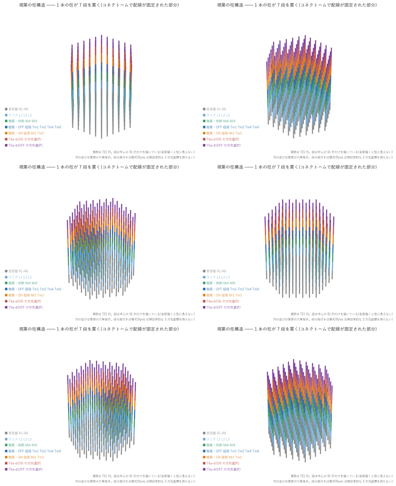
↑ The same optic lobe, rotating in 3-D. The 721 columns keep their arrangement through all seven stages — that is the columnar organisation — with one colour per stage (receptors → lamina → medulla ON / OFF / modulatory → T4, the ON direction-selective cells → T5, the OFF ones). Column positions are the real hexagonal lattice, but the depth between stages is schematic: flyvis is a columns × cell-types network and carries no anatomical 3-D coordinates. When section 5 talks about “folding the degrees of freedom per cell type”, these colours are the unit it folds along.
So what is that measured wiring, concretely? Here it is, drawn.
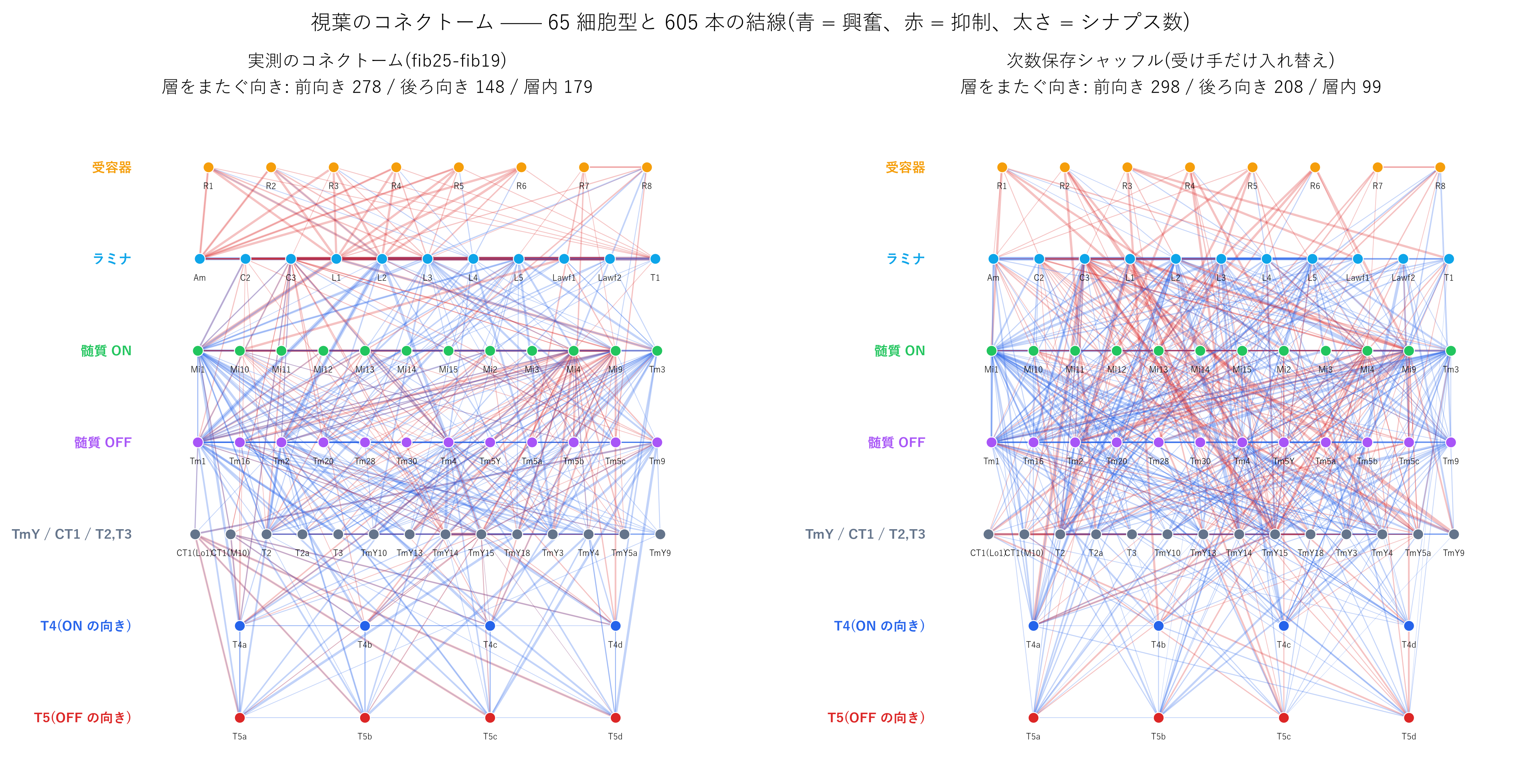
↑ Left: the measured connectome (fib25-fib19; 65 cell types, 605 type-to-type connections). Nodes are cell types, laid out in the order light travels through them. Blue is excitatory, red inhibitory; line width is synapses per receiving cell. Right: a degree-preserving shuffle — every type keeps its in-degree, out-degree and sign, and only the targets are swapped. Same edge count, same degrees, but the direction profile changes: within-layer connections fall from 179 to 99, while backward ones (against the direction of light) rise from 148 to 208. Figure labels are in Japanese.
Those red lines criss-crossing the layers on the right are what the “shuffled-connectome control” later in this article actually destroyed. Same edges, same degrees — the layered structure is not preserved.
So only the optic lobe is genuinely connectome-derived; everything before and after it (eye geometry, readout, behaviour) was written by hand. Every number below describes “the optic lobe wired up this particular way”.
One more thing worth stating plainly: an insect’s central nervous system is not confined to its head. The thorax carries a ventral nerve cord (VNC) of roughly 23,000 neurons, and that is where walking is generated — the brain sends roughly 1,328 descending neurons to it. A decapitated fly can still walk (reported in 1997). When this article says “walking is kinematic”, what it means is that something the VNC would normally produce is hand-written here instead. Brain-plus-VNC connectomes (BANC, MaleCNS) were published in 2026, so this part can get closer to the real thing later.
0. Designing the eye itself — compound-eye optics as closed-form operators
The table above files “the eye” under hand-written. Here is what that hand-written part actually is. A compound eye is a design, and it has exactly three knobs:
- Δφ (inter-ommatidial angle) — how many degrees apart the viewing axes sit. The sampling pitch.
- Δρ (acceptance angle) — how wide a cone one ommatidium integrates over (Gaussian, full width at half maximum). The blur.
- radius — how many you place (n = 3R(R+1)+1; R = 15 gives 721).
Fix those three and what the eye can and cannot see follows from a formula. The flyvision family in Fullseye, my own vision library, implements that path as closed-form operators, so changing the design and re-measuring it takes a few lines.
import flyvision as fv

lat = fv.fly_hex_lattice(radius=15, dphi_deg=4.63, geometry="boxeye")  # 721 viewing axes
sky = fv.fly_sky_1f(width=1440, height=720, amp=0.45, seed=7)          # a synthetic 1/f sky
sig = fv.fly_hex_resample(img, lat, drho_deg=8.23, fov_deg=110)        # what the eye sees: 721 values
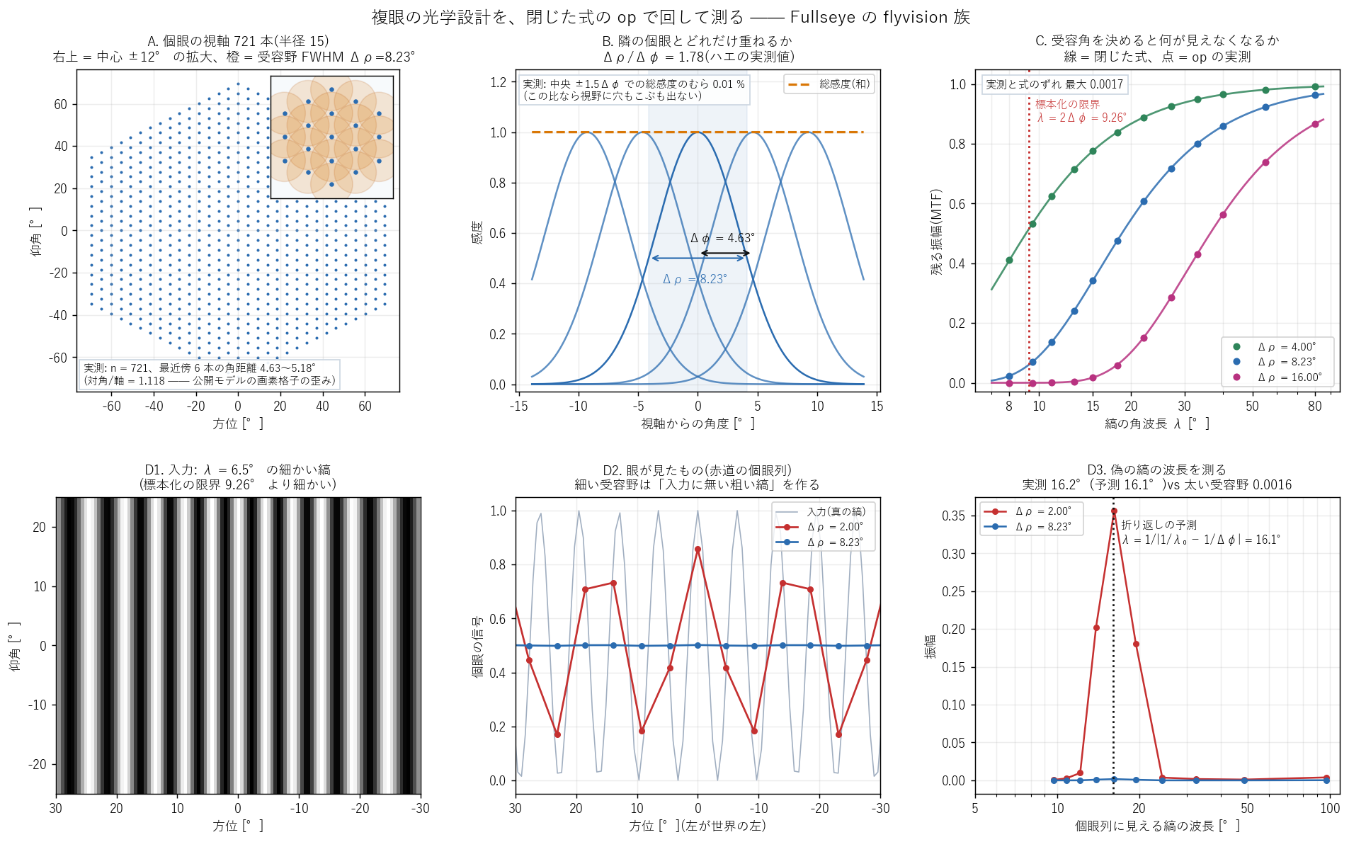
↑ Every panel is the operators actually run — there is no schematic anywhere in this figure. A the 721 viewing axes (inset: the central ±12°, orange = the acceptance width). Matched to the pixel grid of the published model, the diagonal spacing is 1.118× the axial one, and that distortion is reproduced. B how much neighbours overlap. At the fly’s ratio Δρ/Δφ = 1.78 the summed sensitivity ripples by 0.0052 % — no holes and no bumps across the field. C what a given acceptance angle throws away: the line is the closed form exp(−π²Δρ²/(4 ln2 λ²)), the dots are the operator, and they differ by at most 0.0017. D what happens with a grating finer than the sampling limit (λ = 2Δφ = 9.26°).
| D is the part worth stopping at. The input is a 6.5° grating (D1). Narrow the acceptance to 2° and the row of ommatidia reports a coarse ripple that is not in the input at all (red, D2). That is aliasing, and its wavelength is predictable: λ = 1/ | 1/6.5 − 1/4.63 | = 16.1°. Measured: 16.2° (D3). At the fly’s own 8.23°, the same false grating is 223× smaller (0.357 → 0.0016). |
So Δρ/Δφ ≈ 1.8 is not “blurry” — it is the acceptance angle tuned to the sampling limit so that false signal dies. Narrower looks sharper and invents patterns that were never there; wider kills those but dissolves the real ones too (the magenta curve in C).
This section comes first because before blaming the brain for what it could not read, you need to know what the eye already discarded — which is exactly what section 2 turns on. And none of this is fly-specific: change Δφ and Δρ and the same operators design and measure a bee’s eye, or an ant’s.
What follows is not a measurement but a hope. An event-based camera — a sensor whose pixels report brightness changes asynchronously — can be read as a silicon implementation of the very first thing the fly’s visual front end does: drop the DC and send only the change — the lamina’s L1/L2 band-pass. In the Fullseye PoC, skipping that one stage drops the rotation correlation from 0.785 to 0.504: the correlator starts emitting DC × high-pass jitter ten times larger than its mean motion response. If that is right, the part still missing sits one stage earlier, in the optics: a sensor whose inter-ommatidial angle and acceptance angle are design parameters, so that aliasing dies in the device rather than in post-processing. Today’s event cameras are square-gridded, with acceptance treated as an afterthought of the lens. A device that ships with a hexagonal lattice and Δρ/Δφ ≈ 1.8 built in would make the “inventing patterns that were never there” problem of panel D disappear with no downstream computation at all. The fly has shipped that design for half a billion years. If such a sensor appears, the way of measuring in this article moves to real hardware unchanged.
1. It passed every static test, then failed while walking
The first step was to calibrate the optic lobe output by rotating the fly in place. Three tests were built:
- Monotonicity —— does the output increase monotonically with rotation speed?
- Symmetry —— is it symmetric about the origin, left versus right?
- Latency —— is the rise time within a physiological range?
All three passed. The output was monotonic and origin-symmetric up to ±2 rad/s, with a 0.11 s latency (63 % rise). Across places the gain varied by only ±35 % after normalisation. At that point it was tempting to call the sensor usable.
Then the same quantity was read while walking. Correlation across every candidate readout: 0.06–0.51. A complete failure. The three tests that passed had predicted nothing about performance during locomotion.
The reason becomes clear in the next section, but the lesson is already fixed:
Put the test where the accident happens. A verdict obtained from static stimuli says nothing about performance under motion.
This is not specific to flies. A model with good benchmark accuracy that collapses once real motion enters your robot’s camera is the same failure, with the same shape.
2. Measure the world before suspecting the brain
The first suspects were the model (“maybe the pretrained weights do not fit this body”) and the readout expression. Both were wrong.
The cause was the statistics of the stimulus. Optic flow splits into two components:
- Flow from rotation equals the angular velocity itself. It does not depend on distance.
- Flow from translation equals speed ÷ distance. The nearer something is, the faster it streams.
The fly’s eyes sit 1.2 mm above the floor. Even at a walking speed of 2.8 cm/s, the floor directly below streams past at 330–1000°/s — far above the band T4/T5 can follow, burying the rotation signal in noise.
The fix was one line: read only above the horizon. Distant flow has a large denominator, so the translation term vanishes and only rotation survives. Walking self-rotation estimation then reached correlation 0.98.
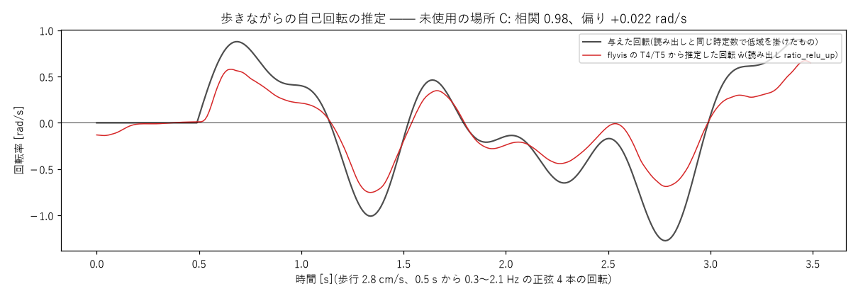
↑ Self-rotation during walking at place C, which was never used for any selection. Black is the imposed rotation, red is the estimate read out from T4/T5. Correlation 0.98, bias +0.022 rad/s — but the amplitude comes out at roughly 0.6× the truth (see section 7). Labels are in Japanese: the axes are rotation rate [rad/s] against time [s].
There is a second trap here. Reading above the horizon helps only if the distant background has texture at all. The first world had a smoothly graded sky, so everything above the horizon was nearly uniform and carried no cue whatsoever. Only after adding a cloud band at 20–60° elevation (1/f in azimuth, amplitude 0.12) did the 0.98 appear. Without the band: 0.06.
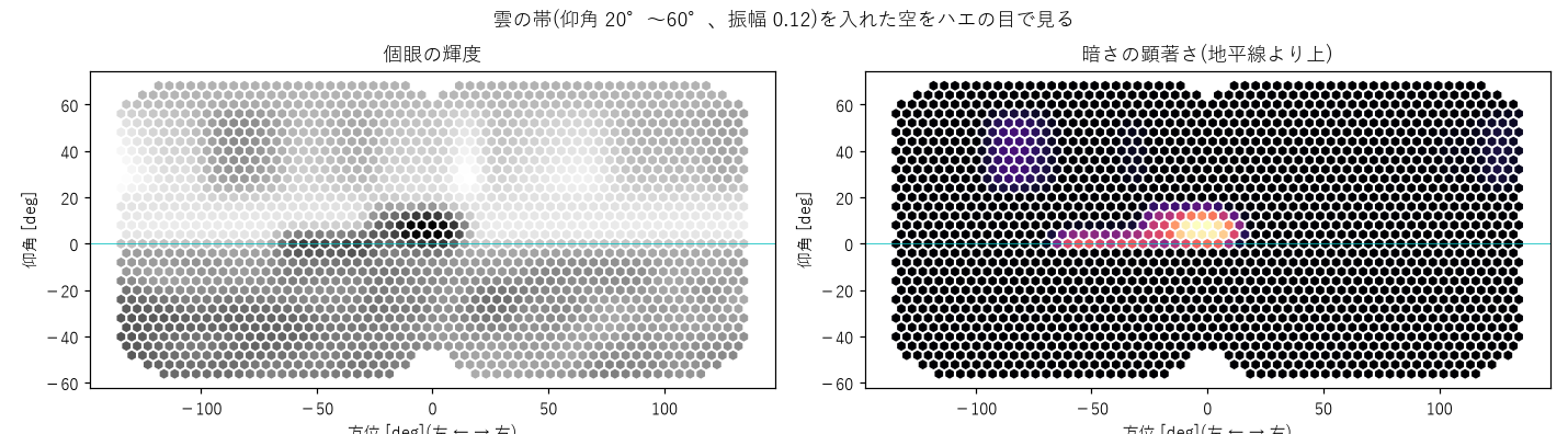
↑ What the compound eye (721 ommatidia, 4.63° between optical axes) sees at that moment. Left: brightness per ommatidium. Right: the salience of “something dark above the horizon”. Whether the sky band exists changes the rotation estimate from 0.06 to 0.98. Figure labels are in Japanese; every number is repeated in the text.
A defect in the world looks exactly like a defect in the brain. Before measuring a model, measure whether the cue exists in the stimulus.
To be honest about it: adding texture to the sky is a convenient modification. The justification is that real outdoor scenes contain clouds, canopies and terrain silhouettes, and a perfectly uniform distance is the unusual case. Still, since the amount of texture was chosen here, 0.98 is a number that includes the world setting — it is not the model’s performance in isolation.
3. Being a good sensor and improving behaviour are different things
With rotation readable, the estimate was fed into steering. Three conditions, twelve runs each:
- Fixation only —— the hand-written “turn towards something darker than the sky”
- + optomotor —— add a steering term opposing the visually estimated rotation
- + efference copy —— subtract the agent’s own commanded turn from the estimate first
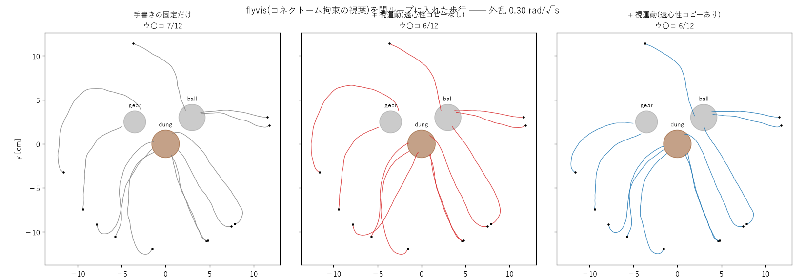
↑ Twelve trajectories per condition. The coloured disc at the centre is the target; grey discs are distractors (gear, lattice sphere). Left to right: fixation only / + optomotor / + efference copy. Arrivals: 7 / 6 / 6.
(Of these three conditions, the one actually moving at the top of this article is “+ efference copy”. The approach to the brown target itself is the hand-written fixation behaviour; the optic lobe only contributes a steering correction — which is exactly the point of this section.)
The result: 7 / 6 / 6. With the disturbance tripled it became 7 / 4 / 6, meaning feedback without efference copy actively hurt (the agent’s own turns were mistaken for disturbance and cancelled).
So a sensor with correlation 0.98 changed behaviour not at all on this task. Fixation dominated; the optomotor path was redundant.
Measure and report sensor fidelity and behavioural success separately. One being good says nothing about the other.
This bears directly on objective design. Optimise for behaviour and the hand-written part wins, leaving the model almost stationary. Optimise for sensor accuracy and it overfits — which is the next section.
4. How much is the wiring actually worth?
The selling point of a connectome-constrained model is that the wiring is measured. So: how many points of performance is that wiring worth? Answering this requires comparing against a classical motion detector on the same stimulus with the same readout.
The comparison is the 1956 EMD (two neighbouring samples, delay one, multiply). It was implemented with operators from a self-built image-processing library, and its parameters (time constants for the delay and the high-pass) were chosen using training places only, leaving C and D unseen.
| Motion detector | A | B | C (held out) | D (held out) |
|---|---|---|---|---|
| EMD on raw luminance (τ 0.05 s) | 0.45 | 0.57 | 0.62 | 0.77 |
| EMD + high-pass (τ 0.1 s, τ_hp 0.2 s) | 0.79 | 0.88 | 0.84 | 0.78 |
| flyvis (connectome-constrained, pretrained) | 0.90 | 0.94 | 0.98 | 0.98 |
Two things follow.
- Preprocessing closes most of the gap. Adding the high-pass stage — the analogue of the lamina, the layer right after the photoreceptors — lifts the EMD from the low 0.6s to the low 0.8s. It is not “the connectome lets it see”; it is mostly removing the slowly varying part of brightness.
- The remaining 0.14–0.20 is the wiring’s share. ON/OFF pathway separation, normalisation and spatial integration earn that. Not zero, but not an order of magnitude either.
That number is directly usable: if 0.84 is good enough for your application, ten lines of EMD will do.
5. More degrees of freedom, less generalisation from little data
Now the main result. Keep the wiring fixed; evolve only the free parameters.
Setup: CMA-ES, 1500 evaluations, step size σ0 = 0.1, objective = correlation of walking self-rotation estimation on the training places. Held-out places C and D are never used for selection.
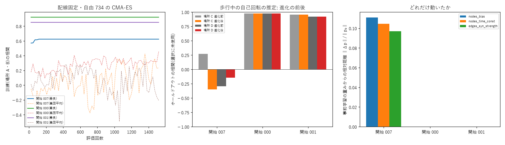
↑ Evolution with two training places. Left: training progress. Middle: held-out score before and after. Right: relative distance travelled from the pretrained weights. Starting point 007 improved on training while its held-out score went negative; starting points 000 and 001 never moved at all (distance 0). Labels are in Japanese; the numbers are all in the text below.
Two things happened.
- Good starting points do not move. Individuals that already generalised (000, 001) produced nothing better than their pretrained point in 1500 evaluations; the distance travelled was exactly 0 — a strong local optimum. Raising the step size to 0.2 destroyed them instead (mean 0.13).
- Bad starting points overfit. Individual 007 went from −0.37 / +0.31 to +0.76 / +0.49 on training, while its held-out scores went from +0.27 / −0.30 to −0.35 / −0.14 — worse than before evolution. It had simply memorised scene features.
Two levers were tried against this.
Lever A: more environments. Raising the training set from 2 places to 10 brought the same 734-dimensional evolution to C 0.887 / D 0.944 on held-out places. The overfitting disappears. A plain result.
Lever B: compress the degrees of freedom. This one is more interesting. The 734 free parameters live “per synapse”. A genome cannot hold per-synapse values — the most it can encode is something like rules per cell type (Zador’s genomic bottleneck, 2019).
So the search variables were folded into 260 dimensions:
- bias per cell type (65)
- log time constant per cell type (65)
- synaptic gain per presynaptic cell type (65)
- synaptic gain per postsynaptic cell type (65)
Each synaptic strength becomes presynaptic gain × postsynaptic gain × pretrained value. Not a single new connection is created (attempting one is a hard failure).
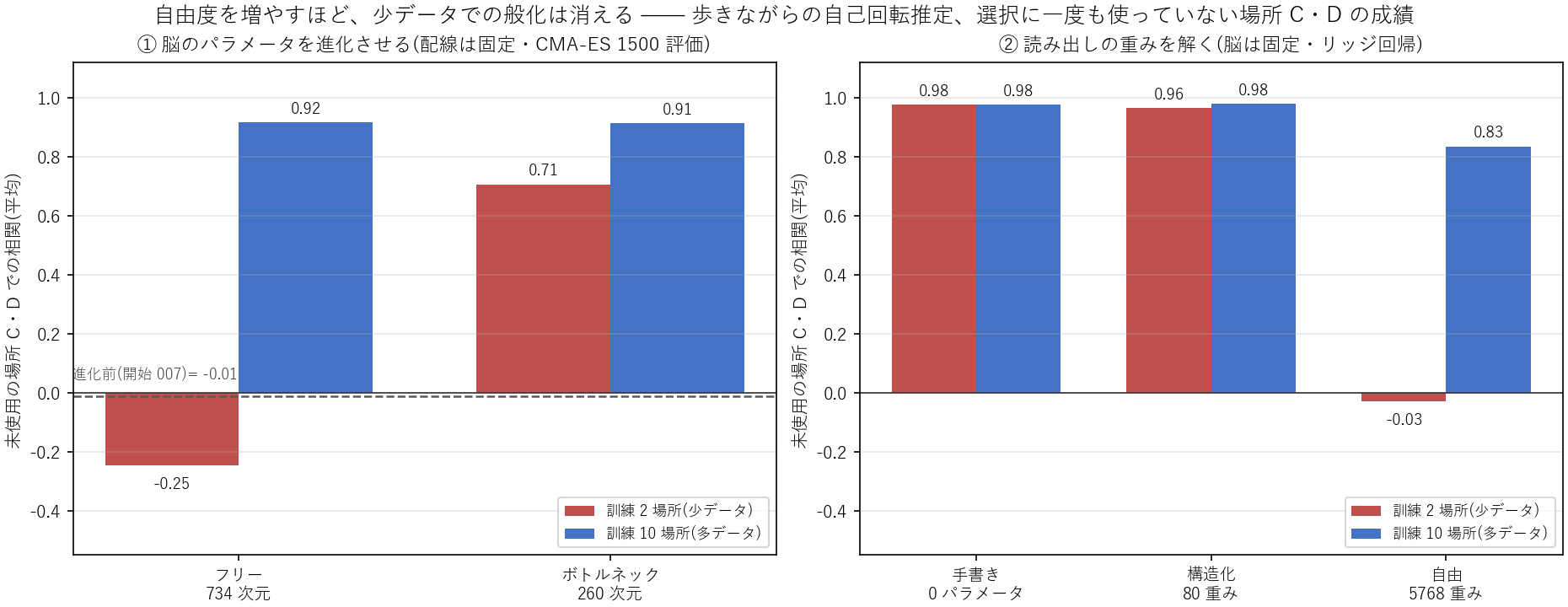
↑ Left: evolution (moving the brain’s parameters). Right: readout (brain frozen, solving linear weights). In both panels the vertical axis is the mean correlation on places C and D, never used for selection. Red is 2 training places, blue is 10. Figure labels are in Japanese; all values appear in the tables below.
In numbers:
| Degrees of freedom | 2 training places | 10 training places |
|---|---|---|
| Free, 734 dims (per synapse) | −0.25 | +0.92 |
| Bottleneck, 260 dims (per cell type) | +0.71 | +0.91 |
Two wins.
- It wins when data is scarce. Same two scenes, same starting point, same evaluation budget: the free search overfits into negative territory while the bottleneck generalises to +0.71. Cutting the degrees of freedom to a third reverses the ranking.
- It ties when data is plentiful. With 10 scenes: free 0.916, bottleneck 0.914. The same generalisation with one third of the freedom.
The same shape appeared without touching the brain at all, by solving the readout side (right panel) — a ridge regression from T4/T5 activity to self-rotation, with λ chosen by leave-one-out on the training places only:
| Readout | 2 training places | 10 training places |
|---|---|---|
| Hand-written (0 parameters) | +0.98 | +0.98 |
| Structured (cell type × elevation band = 80 weights) | +0.96 | +0.98 |
| Free (cell type × column = 5768 weights) | −0.03 | +0.83 |
The 5768-weight fit memorised the scene outright on two places (held-out C 0.13 / D −0.19) and still had not caught up on ten (D 0.72). The 80-weight version, which only pools over elevation bands, reaches 0.96 with two places. Opening up its closed-form weights showed it had rediscovered the structure of the hand-written expression: T4a negative and T4b positive, concentrated in elevation bands 6–8 (exactly where the cloud band sits), essentially zero in the lower half.
An inductive bias wins when data is scarce and costs nothing when it is not — provided the axis you fold along is a real structural unit (cell type, elevation band).
Honest caveats. (a) The hand-written readout already sits at 0.98, so mathematical optimisation buys no performance on this task; what it bought was confirmation that the hand-written form is near-optimal, and an explanation of its structure. (b) The 260-dimensional cut is a design decision about granularity, not a deduction from biology. (c) The 2-place condition starts from 007, a starting point that is particularly bad for the free search; a different start changes the size of the gap.
6. Behaviour improves, biological realism degrades
One more quantity was measured at every step: direction selectivity (DSI) of T4/T5, probed with moving edges at six speeds.
- The solution that overfitted on 2 scenes: 3/8 types selective → 2/8. T4a fell from 0.59 to 0.00.
- The solution that generalised on 10 scenes: training and held-out both improved, yet selectivity went 3/8 → 1/8.
- An individual that already generalised, evolved further: 7/8 → 4/8.
Behavioural performance and biological realism dissociated cleanly. Reading self-rotation, as a single task, does not require T4/T5 to discriminate direction. Indeed, an individual whose T5 cells are almost non-selective still estimates self-rotation at 0.96 — T5 is redundant for this task.
For completeness, the untrained network (wiring only, parameters from the initial distribution) was also measured: direction selectivity 0/8, self-rotation estimation ≈ 0, insensitive to the random seed. The wiring does not supply the function; it supplies the scaffold that makes learning it fast.
Optimise for a single task and every property that task does not need will be removed. To keep a property, include a task that requires it.
7. Closing the loop: see → orient → move
Finally, the visual estimate was connected to navigation. The insect central complex contains a ring attractor representing heading (a bump travelling around a circle) and a path integrator accumulating the home vector. Both were implemented with closed-form checks (bound on phase error, closed-loop residual, monotonic approach on the homeward leg), and the flyvis angular velocity estimate was fed into the compass.
Correction (2026-09-15): the numbers in this section (7.4 / 23.5 / 19.8 %), the “error decomposition” and the “circling” explanation are retracted. The ring attractor had been used without calibration (second entry in §8). The calibrated numbers and the deceleration experiment are in the appendix, “Homing with deceleration”. The original text and figure are left as they were.
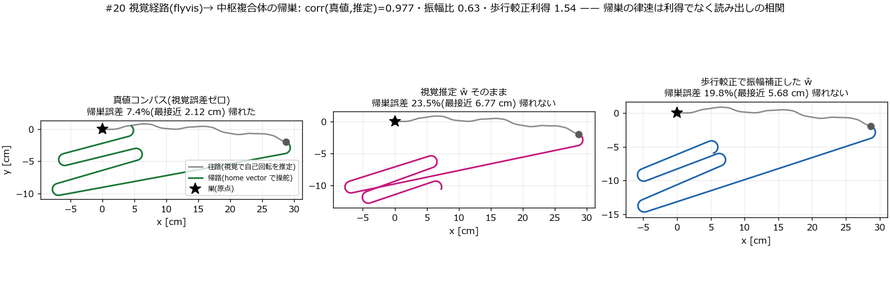
↑ The first-version figure (uncalibrated compass). Left: a ground-truth compass (zero visual error). Middle: the raw visual estimate. Right: the visual estimate with its amplitude corrected by a walking calibration. Grey is the outbound path, colour is the homeward path, the star is the nest. Labels are in Japanese; the error percentages are in the text.
- Ground-truth compass: homing error 7.4 % (closest approach relative to a 28.8 cm outbound path)
- Raw visual estimate: 23.5 % (does not get home)
- Amplitude calibrated: 19.8 %
The visual estimate has only 0.63× the true amplitude, so naively multiplying by 1.54 ought to fix it. It does not — calibration recovers only as far as 19.8 %. Decomposing the error:
- due to the amplitude mismatch: 3.8 points
- due to residual noise behind a correlation of 0.977: 12.4 points
The residual dominates by 3.4×. Path integration accumulates error, so even an instantaneous correlation of 0.977 matters after a few seconds. In other words, the next effective lever is not calibration but raising the readout correlation itself — which ties this section back to the previous ones: environment diversity, compressed degrees of freedom and staged task curricula all feed straight into homing accuracy.
The 7.4 % that remains even with a perfect compass comes from holding forward speed constant, which makes the agent circle over the nest. Insects decelerate on approach; adding deceleration interferes with the memory update, so that needs its own experiment.
8. A retracted result
One conclusion here was wrong and has been withdrawn.
In an experiment that enlarged the eye (721 → 1951 ommatidia, same pretrained weights), the first write-up said: “if you add ommatidia without narrowing the acceptance angle, performance collapses — the optics must co-adapt.” A plausible story, and the numbers did collapse (correlations −0.11 to 0.45).
The cause was not optics. It was a tooling defect in which the second eye constructed inside the same process rendered a broken image — the giveaway was near-zero variance across columns and a comparison EMD returning nan. Rebuilt in a separate process, the same configuration behaved normally (0.96–0.99).
What actually holds: enlarging the eye does not break anything even without retraining; it improves slightly and saturates (0.98 → 0.98–0.99). Shrinking (331 ommatidia) does hurt. Acceptance-angle co-adaptation does not matter over this range.
When a result surprises you, suspect tool ordering before you reach for physics. The second object built in one process, the second call to a function, the second run that hit a cache — reproduce it in isolation before interpreting it.
Second retraction (2026-09-15). The homing numbers in §7 (ground truth 7.4 % / raw visual 23.5 % / amplitude-corrected 19.8 %) and what was drawn from them — “the error splits into 3.8 points of amplitude and 12.4 points of residual” and “the 7.4 % is the agent circling at constant speed” — are withdrawn. The ring attractor had been used without calibration, and its bump travelled 10.8 % faster than the angular velocity. Calibrated, the numbers are 1.7 % / 2.1 % / 12.4 %: the raw visual estimate gets home on its own, and the amplitude correction makes things worse (appendix, “Homing with deceleration”). The direction of the conclusion — the residual is what limits homing — survived, but every number that supported it has been replaced. It was found by the deceleration experiment: the agent stopped 9 cm from the nest, I almost called that “interference”, and the cause turned out to be calibration.
Check that a component was calibrated on the caller’s side, not the component’s. A calibration function existing and being called on this path are two different things. §7 used a calibratable part without calibrating it.
What to take away
Folded into forms that survive without the author, there are six:
- Put the test where the accident happens. A verdict from static stimuli does not predict performance under motion.
- Measure the world before suspecting the brain. If the cue is absent from the stimulus, no model can read it — and any performance number includes the world’s settings.
- Report sensor fidelity and behavioural success separately. One says nothing about the other.
- Cut degrees of freedom along structural units. Variables folded per cell type or per elevation band win when data is scarce and cost nothing when it is not — provided the fold matches real structure.
- Single-task optimisation deletes every property the task does not need. Include a task that needs what you want to keep.
- Surprising results: suspect tool ordering before physics.
None of these are specific to flies. They appear whenever someone else’s pretrained model is mounted in your own system.
What was not measured
- Walking is kinematic. There is no leg dynamics, so image motion from ground reaction forces and slipping is absent.
- Everything downstream of the optic lobe (LC cells, descending pathways, motor commands) is hand-written. This is not “a fly brain steering”.
- In the experiment that silences cell types stage by stage, the selectivity index reads 0.0 even when the response is identically zero, so “lost selectivity” and “no response at all” are not distinguishable. Response magnitude per type has to be checked separately; that check is not done yet.
- Evolution was run mostly from starting point 007, an individual that does not generalise. A different starting point changes the size of the effects.
- The connectome constrains the optic lobe, not the whole brain.
- Screening 50 pretrained individuals found zero of the top ten with direction selectivity in all 8 T4/T5 types (one had 7). Two had their T4 directions inverted by a full 180°. “This model reproduces direction selectivity” carries a large individual variance — screen before you use it.
Public models and papers this rests on
- flyvis —— the connectome-constrained optic lobe model (Lappalainen et al., 2024): wiring, synapse counts and signs fixed from measurement, continuous values learned on a task. This is the “optic lobe” here.
- flybody —— the full-body Drosophila physics model (Vaxenburg et al., 2025), supplying body, joints and eye cameras.
- Hassenstein & Reichardt (1956) —— the elementary motion detector, used here as the null baseline.
- Stone et al. (2017) —— an anatomically constrained path integration model of the bee central complex; section 7 follows its structure.
- Zador (2019) —— the genomic bottleneck, the basis for folding per cell type in section 5.
What this PoC uses from Fullseye, and what it gives back
The visual front end is built from the flyvision family (8 operators) in Fullseye, my own vision library. Every one of them is closed-form and ships with a ground-truth test:
| op | role | where it appears here |
|---|---|---|
fly_hex_lattice |
hexagonal viewing axes (n = 3R(R+1)+1) | §0 panel A — the eye’s geometry |
fly_hex_resample |
Gaussian acceptance onto the ommatidia | §0 panels C and D (MTF, aliasing) |
fly_sky_1f |
synthetic sky with a 1/f band | §2, “texture in the distance” |
fly_emd_response |
Hassenstein–Reichardt correlator | §4, the zero point |
fly_hs_readout |
wide-field opponent sum (HS-like) | the shape of the readout |
fly_dsi |
direction selectivity index | §6, the 8-type test |
fly_lgmd_eta / fly_tau_from_expansion |
looming (η and time-to-contact τ) | unused here — measurable from the same eye |
What goes back into Fullseye is two things. (1) A measurement bench: swap the motion detector and the stimulus, readout and scoring stay identical — which is the only reason section 4’s question (“how many points does a connectome-constrained model add over the textbook formula?” → 0.14–0.20) can be answered at all. Existing implementations can run a model; they are not built to line it up against a different detector on the same stimulus. (2) Counter-examples: the aliasing in §0 and the floor flow in §2 come back as a concrete demand — lift the operators’ tests from “a static synthetic image” to “measured while walking”.
Conversely, the body, the physics and the connectome model stay external dependencies (flybody / flyvis), and there is no plan to reimplement them. The value is in the bench you mount them on.
Appendix: later experiments
Where flies and vertebrates do the same job (2026-09-14)
“Which part of a human brain is this?” is a natural question. But the last common ancestor of insects and vertebrates lived 550 million years ago, and their visual circuits share no cell lineage. So every answer below is convergence, not homology — two lineages arriving at the same solution separately. Only correspondences that could be checked against primary literature are drawn.
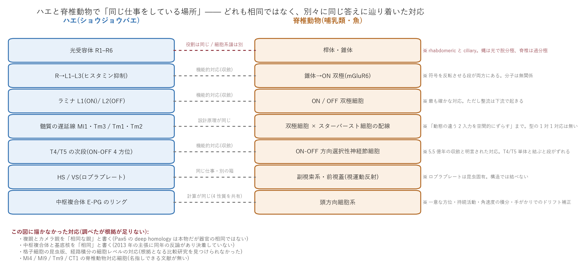
↑ Fly on the left, vertebrate on the right. A dotted line means “a correspondence that is not homology.” The red row (photoreceptors) shares a role but not a lineage — and the response polarity is opposite as well: fly photoreceptors depolarise to light, vertebrate rods and cones hyperpolarise. The safest correspondence is L1 (ON) / L2 (OFF) with ON / OFF bipolar cells; the strongest computational match is the central-complex ring with the head-direction system, where a ring attractor has been measured on both sides. The lower right lists what was researched and then deliberately left out — an insect version of grid cells, or homology between the central complex and the basal ganglia, would be speculation. Figure labels are in Japanese.
This reframes the first half of the article slightly. Splitting ON from OFF in the lamina, multiplying two inputs of different dynamics offset in space, then pooling the result in wide-field cells to stabilise posture — none of that is “how flies do it”. It is a design adopted twice, independently, across 550 million years. The 0.14–0.20 measured in §4 is then the premium that having that design in measured wiring buys over writing the textbook equation yourself.
Shuffling the wiring changed nothing — and “nothing” is not what I get to write (2026-09-14)
§4 measured the wiring’s share by swapping the wiring underneath pretrained weights: 0.14–0.20. This is the harder version of that question. From the same untrained initialisation, evolve the real wiring and two degree-preserving shuffles of it on the same task with the same budget (734 dimensions, 1500 evaluations, about three hours per condition). Starting untrained removes the confound of the pretrained point.
| Condition | Train | Held-out mean | C | D |
|---|---|---|---|---|
| Real wiring | +0.196 | +0.171 | −0.292 | +0.633 |
| Shuffle 0 | +0.205 | +0.198 | −0.138 | +0.535 |
| Shuffle 1 | +0.145 | +0.039 | −0.215 | +0.294 |
Real minus the shuffle mean is +0.052 on held-out scenes. But the two shuffles differ from each other by 0.159 — three times that. This experiment does not have the sensitivity to measure what it was built to measure.
Worth recording is where this nearly went wrong. With only the first shuffle finished, the numbers said the shuffle was slightly better (−0.028) — exactly the shape that invites writing “the wiring is worth nothing”. The second shuffle flips the sign. At n = 1 you cannot trust the magnitude of a difference, and you cannot trust its sign either.
Three reasons the sensitivity is missing. (1) The search had effectively collapsed to biases alone. Normalising each tensor by its standard deviation drove the scale to 3.75e-09 for a near-constant initialisation (all time constants start at 0.05), and the guard only tested std > 0, so it sailed through. In all three conditions the time constants moved by 1e-8 — not at all. An effective floor now fixes this, but the three runs above are from the old code, so the caveat stays. (2) One seed per condition: no error bars. (3) As §6 shows, direction selectivity is 0/8 before training — wiring alone produces no function, so any difference due to wiring may be swamped by differences in learning before it can appear.
The next step is not to write a conclusion; it is to raise the sensitivity — floored scales, at least three seeds per condition, and more shuffles.
A staged curriculum can build direction selectivity — and the last stage destroys it (2026-09-14)
§6 reported that optimising for behaviour alone breaks direction selectivity — the property that makes T4/T5 discriminate motion direction. The obvious countermeasure is to demand discrimination explicitly, in stages: brightness → ON/OFF → direction → rotation, 400 evaluations each, every stage starting from the previous stage’s solution. Two starting points were run.
| Stage | From untrained | From the trained start (007) |
|---|---|---|
| S1 brightness | 0.353 | 1.000 |
| S2 ON/OFF | 0.796 | 0.964 |
| S3 direction (DSI) | 0.002 | 0.377 (5 of 8 types pass) |
| S4 rotation (M4) | 0.061 | 0.799 (held-out C 0.823 / D 0.811, 1/8 pass) |
Two things follow.
(1) The curriculum can build direction selectivity — but only from a trained starting point. From 007 the direction stage takes it from 0/8 to 5/8. From the untrained start, four stages of climbing leave it at 0/8, and the direction stage itself scores 0.002 — no climb at all. Wiring is the scaffold, but you cannot climb the scaffold alone. That is the same statement as the shuffle appendix above and as §6’s “0/8 before training”, arrived at from a third direction.
(2) What the curriculum builds, the final behavioural stage destroys. The 5/8 earned in the direction stage falls to 1/8 once the rotation stage is learned — while rotation estimation itself climbs to 0.82 on scenes never used. The performance-versus-realism trade-off is running inside a single search, over time. Earlier stages decay too (ON/OFF 0.874 → 0.536).
The remedy is known — make stage k’s objective the mean over stages 1…k. It has now been run; the result is in “Forgetting disappeared when the objective was written differently” below — point (2) of this section is one I go on to overturn myself.
One more thing: this is the first experiment to run after the scale collapse described above was fixed. Its report file records “the time-constant scale was 3.75e-09, so the floor of 0.001 was used” — the fix is visible in the output, not just in the diff.
Looking at the fly’s own world through other sensors (2026-09-14)
§0 designed the optics. Here is what that eye actually sees: the walk replayed, rendered from the eye camera that the published Drosophila model already carries (140° field of view).
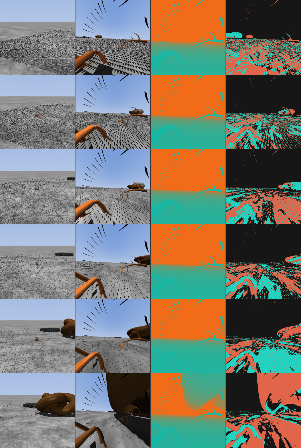
↑ From the left: ① the fly in its world (the small orange dot at centre), ② the view from its compound eye (the thick bars in front are its own legs, the black combs above are the antennae, the mass past the horizon is the target), ③ depth (blue-green near → amber far; the sky is excluded from the colour range), ④ synthetic events (pixels that brightened in blue-green, pixels that darkened in red). One viewpoint, three sensors, at once.
Panel ④ connects back to §0. As the fly advances, the floor texture streams outward from below and shows up as events — the same flow that §2 measured at 330–1000°/s, past the passband of the motion detectors. An event camera transmits only change, so that flow is the sensor’s output.
And the interference pattern on the floor in ① and ② is not a rendering defect — it is the aliasing measured in §0. The floor texture is finer than the pixel spacing, so the renderer’s sampling invents a coarse pattern that is not there. Exactly what D3 predicted and measured by wavelength, happening in an ordinary render: any eye that tries to see detail finer than it samples will manufacture detail that does not exist.
Honest notes: the body’s trajectory is the real one the closed loop produced, but the leg motion is a cosmetic tripod gait — it is not walking by leg dynamics (as the first table in this article says). Depth and events are synthesised from the render, not the output of a physical sensor.
Which layer, when silenced, breaks self-rotation estimation (developmental ladder, 2026-09-15)
Silencing the visual pathway stage by stage, from the bottom up, and lining up where self-rotation estimation (M4, §5) breaks. 34 conditions — a control, photoreceptors R1–R6, lamina L1–L3, nine medulla Mi/Tm types, T4/T5 in four directions each, and six bundled stages. Each condition pins the output of the named cell types to zero and measures 12 scenes on the same stimulus. Eight threads, 3 h 23 min, 34/34 completed.
| Stage silenced | Worst condition | Correlation | Drop from control |
|---|---|---|---|
| (control) | none |
0.9487 | — |
| Photoreceptors R1–R6 | R6 | 0.5742 | 0.375 |
| Lamina L1–L3 | all, bundled | 0.4853 | 0.463 |
| Medulla Mi/Tm | all, bundled | -0.0057 | 0.954 |
| T4/T5 | T4, bundled | 0.5182 | 0.431 |
Self-rotation estimation is concentrated in the medulla. Drop that layer entirely and the correlation falls to -0.0057 — essentially no correlation. Dropping photoreceptors, lamina or T4/T5 costs only 0.37–0.46 by comparison. Among single cell types, Mi1 (0.031) and Mi4 (0.064) matter most — both ON-pathway relays. T4/T5 are the textbook carriers of direction selectivity, yet for rotation estimation they are not individually decisive. 24 of the 34 conditions fell at least 0.01 below the control.
But only half of this experiment measured anything. Direction selectivity (DSI) was not measurable in all 34 conditions — about 4 million of 10.09 million response elements were non-finite. And since even the control, with nothing silenced, went non-finite, the cause is not the silencing but the response generation itself. The fix made last time — record a condition as “not measurable” and carry on — only made the failure report correctly; it did not fix the non-finite values. A fix landing is not the same as an experiment working.
One lesson. Ride two metrics on a single run and one metric’s failure invalidates every condition. M4 came back 34/34; DSI was lost 34/34. Metrics should run independently, or at minimum the control condition should establish that the metric itself is sound before the sweep starts.
Addendum (same day, afternoon) — what the non-finite values were. The smallest reproduction (model 000, nothing silenced, no hook registered, just two speeds, 19 and 25) shows the speed-25 responses going non-finite from frame 465 on, with zero non-finite values inside the frames where the stimulus itself is finite. The primary source is flyvis’s moving_bar.py, _resample: stimuli of different lengths per speed are padded to the slowest one’s length with NaN (the code says so in a comment), and the network carries the NaN forward with the layer delays. At six speeds that is 62,616 elements per column, structurally — matching the control’s 4,057,080 of 10,090,080 in the full run, and explaining why silenced conditions had exactly 62,616 fewer. flyvis’s own DSI reads only its time window and is unaffected; what was broken was the ladder’s “every element finite” gate. A smoke test at speed 19 alone has no padding, so it could never have found this. The gate now checks only frames where the stimulus is finite; the selftest matches the stored references for all eight cell types with ΔDSI 0.0000. The 34-condition ladder goes back into the queue, DSI included. Lesson: a “must be finite” gate raises false alarms unless it knows where the tool uses NaN on purpose.
Forgetting disappeared when the objective was written differently (2026-09-15)
The previous section reported that a staged curriculum can build direction selectivity but that the final behavioural stage destroys it (5/8 → 1/8). The proposed remedy — the cumulative objective, where stage k is scored as the mean over stages 1…k — has now been run from the same starting point, with the same budget and the same tasks.
| Stage | Contrast | ON/OFF | Direction | Selectivity passing |
|---|---|---|---|---|
| S1 | 1.000 | 0.372 | 0.123 | 1/8 |
| S1+S2 | 1.000 | 0.997 | 0.056 | 1/8 |
| S1+S2+S3 | 0.987 | 0.979 | 0.365 | 4/8 |
| S1+S2+S3+S4 | 0.999 | 0.961 | 0.392 | 6/8 |
Rotation estimation at the final stage, on scenes never used: 0.875 / 0.814.
The forgetting is gone — and behaviour did not pay for it. Staging alone (non-cumulative) ended with selectivity at 5/8 → 1/8 and ON/OFF at 0.874 → 0.536. With the cumulative objective, selectivity goes 4/8 → 6/8 — it increases — and ON/OFF holds at 0.979 → 0.961. Rotation estimation matches or beats the earlier run (0.823 / 0.811).
So the performance-versus-realism trade-off was not a law; it was a way of writing the objective. The previous section’s observation was right as a phenomenon, but I had not read the cause correctly — what broke it was not keeping the property I wanted in the final stage’s objective.
The cost is explicit. Each evaluation measures every stage, so the final stage takes 239.8 s per generation — about 7× the non-cumulative run, 140 minutes in total against roughly 40. Evaluation gets heavier in proportion to how many properties you insist on keeping, which makes “what do we keep” a design decision to be made out loud.
Homing with deceleration — both things that looked like “interference” were something else (2026-09-15)
§7 ended with “adding deceleration interferes with the memory update, so that needs its own experiment”. Running that experiment showed not interference but that the numbers in §7 were wrong.
| First: the compass had not been calibrated. With deceleration (forward speed = v0 · | H | / r_slow, where | H | is the length of the home vector the memory decodes — nothing the brain does not have), even the ground-truth compass stopped 31–41 % of the outbound distance from the nest (worse than the constant-speed 7.4 %), while the memory said “home” and the true position was 9 cm away. Tracing it back: the ring attractor in §7 had been used with its default gain (g = 1), and its bump travelled 10.8 % faster than the angular velocity (1.000 after calibration; the pure time lag is 0.002 rad). The first homeward turn of ≈ π rad puts it 0.34 rad off. Re-measuring §7 with the compass calibrated: |
| Condition | §7 as first published (uncalibrated) | Calibrated |
|---|---|---|
| Ground-truth compass | 7.4 % | 1.7 % (home) |
| Raw visual estimate | 23.5 % (not home) | 2.1 % (home) |
| Amplitude corrected by gain 1.54 | 19.8 % | 12.4 % (worse than raw) |
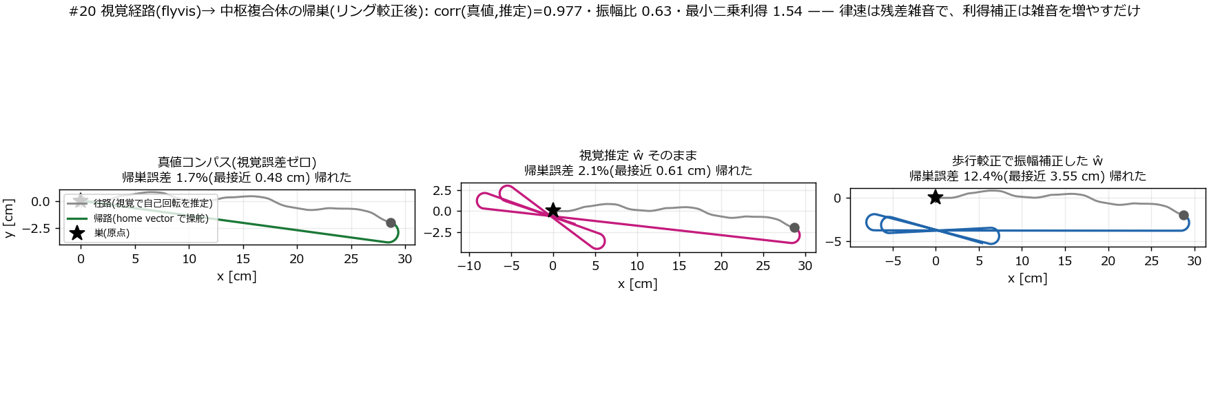
↑ §7 after calibration. The raw visual estimate gets home (middle). The amplitude correction throws the homeward leg off (right).
§7’s “3.8 points amplitude + 12.4 points residual”, “the lever is correlation, not calibration” and “the 7.4 % is circling” were all products of that missing calibration and are retracted (second entry in §8). The calibrated reading: the 0.63× amplitude only matters through the net rotation (−0.26 rad on this outbound path, against 4.6 rad of total turning), whereas the least-squares gain of 1.54 also amplifies the part of the noise that accumulates into heading: the instantaneous residual (std) falls from 0.226 to 0.119 rad/s, but the integrated heading error ∫(ŵ − ω)dt rises from 0.124 to 0.210 rad rms, and the memory error at the turning point from 2.8 cm to 5.3 cm. Path integration only cares about the latter. What decides homing is the residual that accumulates into heading, not the amplitude — the conclusion points the same way, but the numbers behind it are different ones.
| Second: an unstable equilibrium in the rule. With the compass calibrated, deceleration ran away at exactly r_slow = 2 cm, stopping 6.9 cm out. Not a measurement hole but a hole in the rule: steering w = k | H | sin ε (ε the angle to the nest from the heading) and speed both scale with | H | , so the path curvature w / v does not depend on | H | at all — **the moment the agent comes to rest facing away from the nest (sin ε ≈ 0) it does not turn, walks straight off at the speed its residual memory error dictates, and the further it walks the larger | H | gets and the faster it goes** (exponential, time constant r_slow / v0). Which r_slow triggers it depends only on the heading at the moment of stopping; 2 cm was luck. Adding “walk only while the nest is ahead” (multiply v by max(0, cos ε) — the fly’s body saccade: no walking mid-turn) stops it at every r_slow: 0.03 cm for the ground-truth compass, arrival time monotonic in r_slow (10.8 → 25.1 s), and for the visual conditions the stopping error, 0.59 cm (raw) / 3.81 cm (gain-corrected), coincides exactly with the error the memory holds at the moment of stopping. |
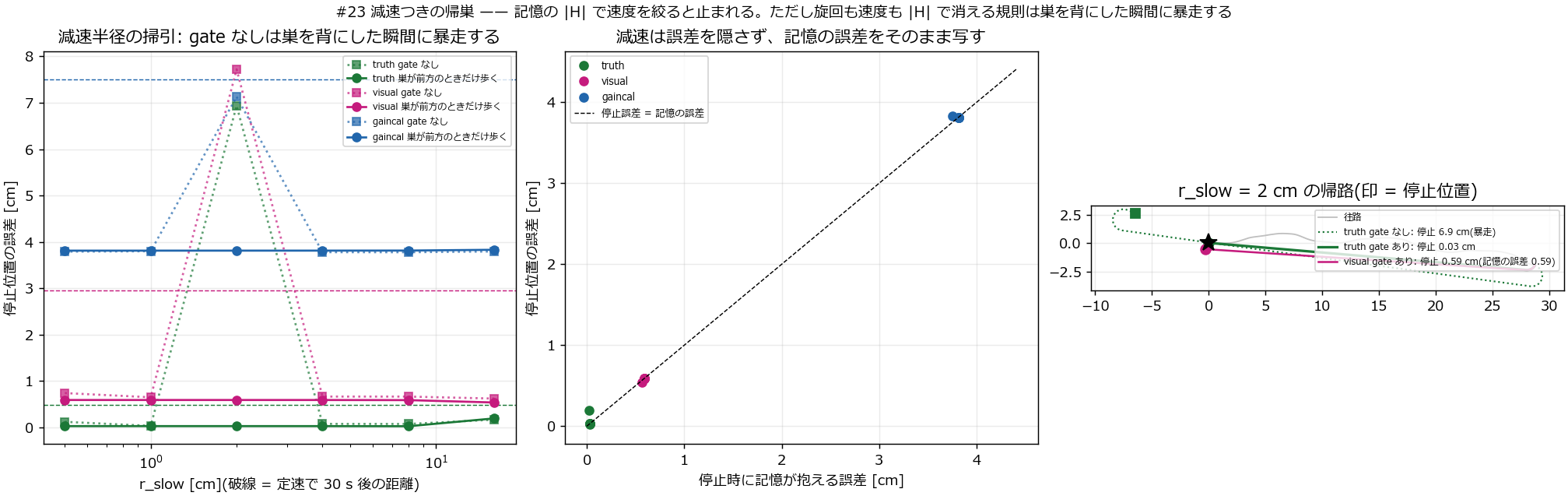
↑ Left: sweep of the deceleration radius r_slow. Dotted (no gate) runs away at 2 cm; solid (walk only while the nest is ahead) stops everywhere. Dashed lines: distance after 30 s at constant speed. Middle: stopping error against the memory’s own error at the stop (on the identity line). Right: the homeward leg at r_slow = 2 cm (markers are the stopping points). Labels are in Japanese.
Deceleration does not interfere with the memory update. Deceleration hides nothing: it writes the error accumulated in memory straight into the stopping position — and since the constant-speed “closest approach” was an optimistic number (the track happened to pass near the nest), deceleration is the more honest metric. The experiment ran four times and three of its pre-registered predictions failed; the record is kept in the script’s docstring.
What we measure next
When a result lands, it gains a row in “Experiments so far” and loses its line here.
- Re-run the developmental ladder with DSI —— the non-finite values were flyvis’s NaN padding of the stimulus; the gate is fixed (addendum above). 34 conditions × 6 speeds, about 3.5 hours.
About the author
The questions and the direction are mine; implementation, sweeps, added controls and the checks that disproved my predictions were delegated to Claude Code. Section 8 records one of those disproofs.
These experiments were run together with Claude Code. I set the questions and the direction; Claude Code did the implementation, the sweeps, the management of long overnight jobs and the adversarial checks. If you want to try it, this invitation link gives you a one-week free trial: claude.ai/referral/0sqPw8E_lw
“I mounted a pretrained model in my own system, it passed the static tests, and it fell over in production” — that is the story I most want to hear from you. A like or a stock helps decide which experiment gets written up next.