fullseye
The Optical-Design and Inspection Wing — exhibit captions
Regenerate the figures with py -3.11 tools/gen_wingopt_gallery.py (one exhibit at a time with --exhibits <name,...>).
Every number burnt into a figure was measured by actually calling optics / visiondesign / defectgen / visionlab, and the results are deterministic (--verify checks the SHA-256 matches).
The one road from design to verdict
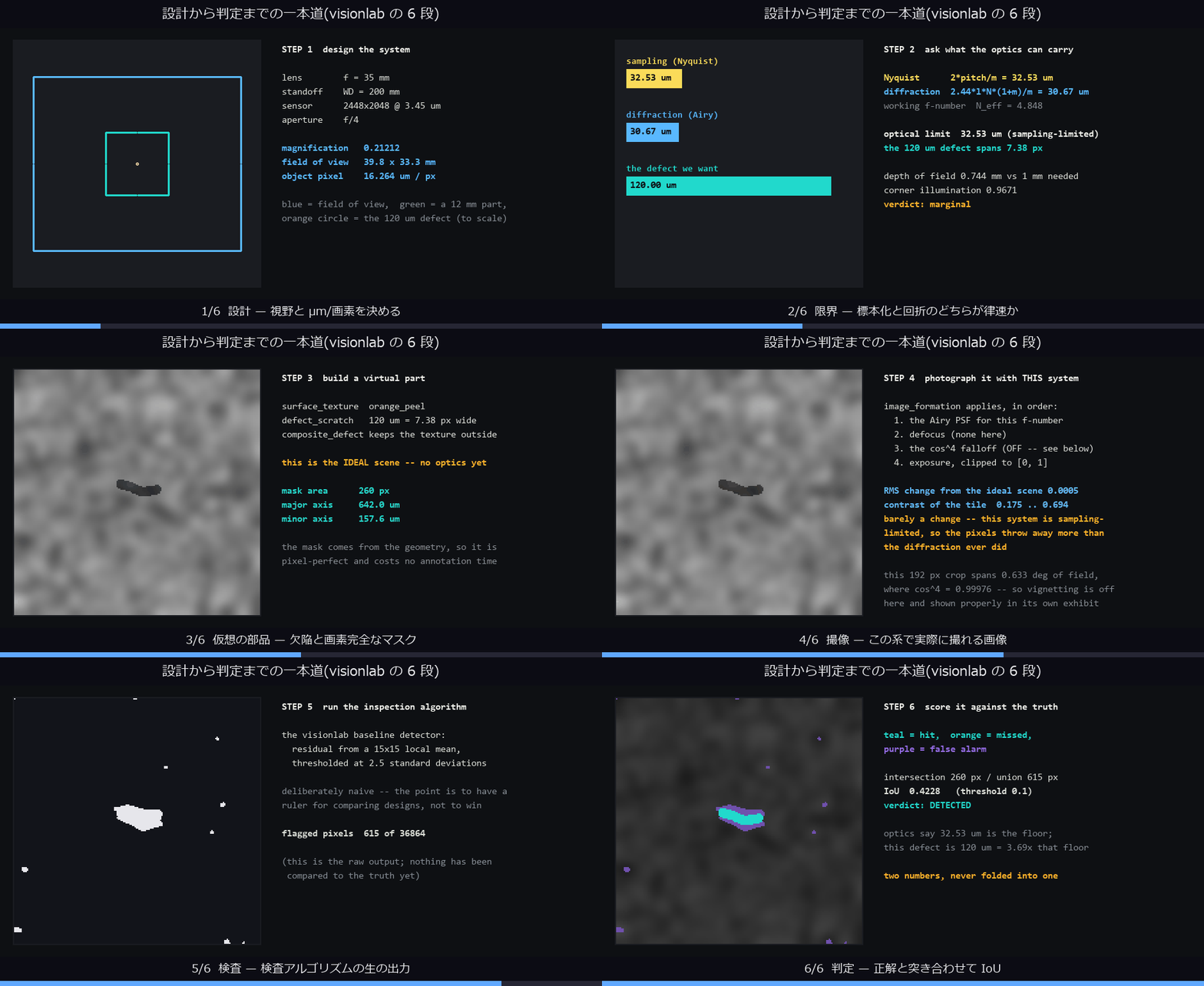
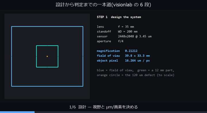
↑ The one road from design to verdict — 6 steps, “design → limit → virtual part → capture → inspect → verdict”, cut into frames you can stop on 1 at a time. Fixing the system fixes 16.264 µm/pixel, out of which comes an optical limit of 32.53 µm (sampling-bound); a 120 µm scratch is then 7.38 pixels, and at the end an IoU of 0.4228 calls it detected — the scoring works because the ground-truth mask does not move when the capture blurs it (the verdict is marginal). Ops used: system_geometry, resolving_power, system_feasibility, surface_texture, defect_scratch, composite_defect, defect_stats, image_formation, draw_polyline, draw_circle.
A single frame still reads (still thumbnail: wingopt_pipeline_flow_thumb.jpg). 6 frames / 700 ms per frame / 940×514 px / 0.30 MB.
A sample book of the defect generator
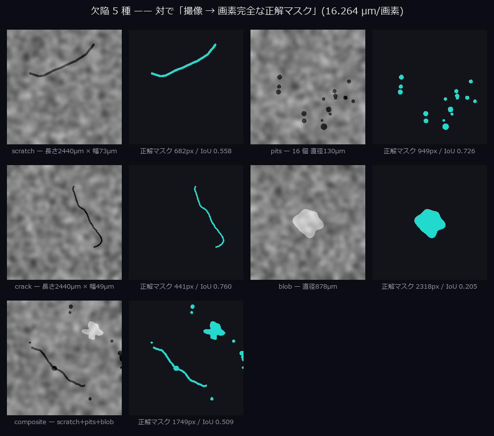
↑ A sample book of the defect generator — 5 defect kinds (scratch / pits / crack / blob / composite) captured through the same system (16.264 µm/pixel); the left column is what the camera sees, the right column is the pixel-exact ground-truth mask. The mask is built from the geometry *before capture, so blur never moves the truth and there is no annotation work at all — the mask areas measure 682 / 949 / 441 / 2318 / 1749 pixels row by row, and the optical limit is 32.53 µm (sampling-bound). Ops used: defect_scratch, defect_pits, defect_crack, defect_blob, surface_texture, composite_defect, defect_stats, image_formation.*
Click for full size (998×882 px / 146 kB).
The limits change places
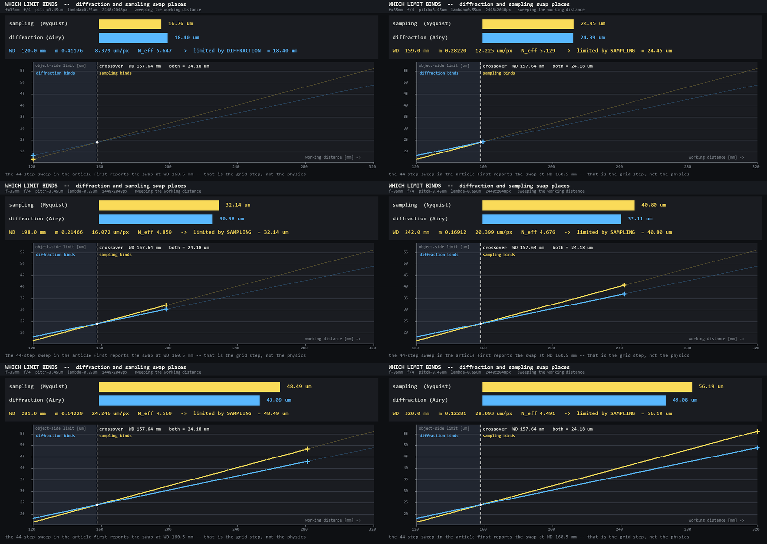
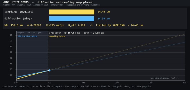
↑ The limits change places — sweep the working distance from 120 to 320 mm and the diffraction limit and the sampling limit swap over. Solved in closed form the crossing sits at WD 157.64 mm, where both limits agree at 24.18 µm (magnification 0.28539). The 44-step sweep in the article body first reports the swap at 160.5 mm — that gap is not physics, it is the coarseness of the grid. Ops used: system_geometry, resolving_power, thin_lens, draw_polyline, draw_line.
A single frame still reads (still thumbnail: wingopt_limit_crossover_thumb.jpg). 42 frames / 10 fps / 1000×474 px / 0.46 MB.
The cos⁴ law of relative illumination
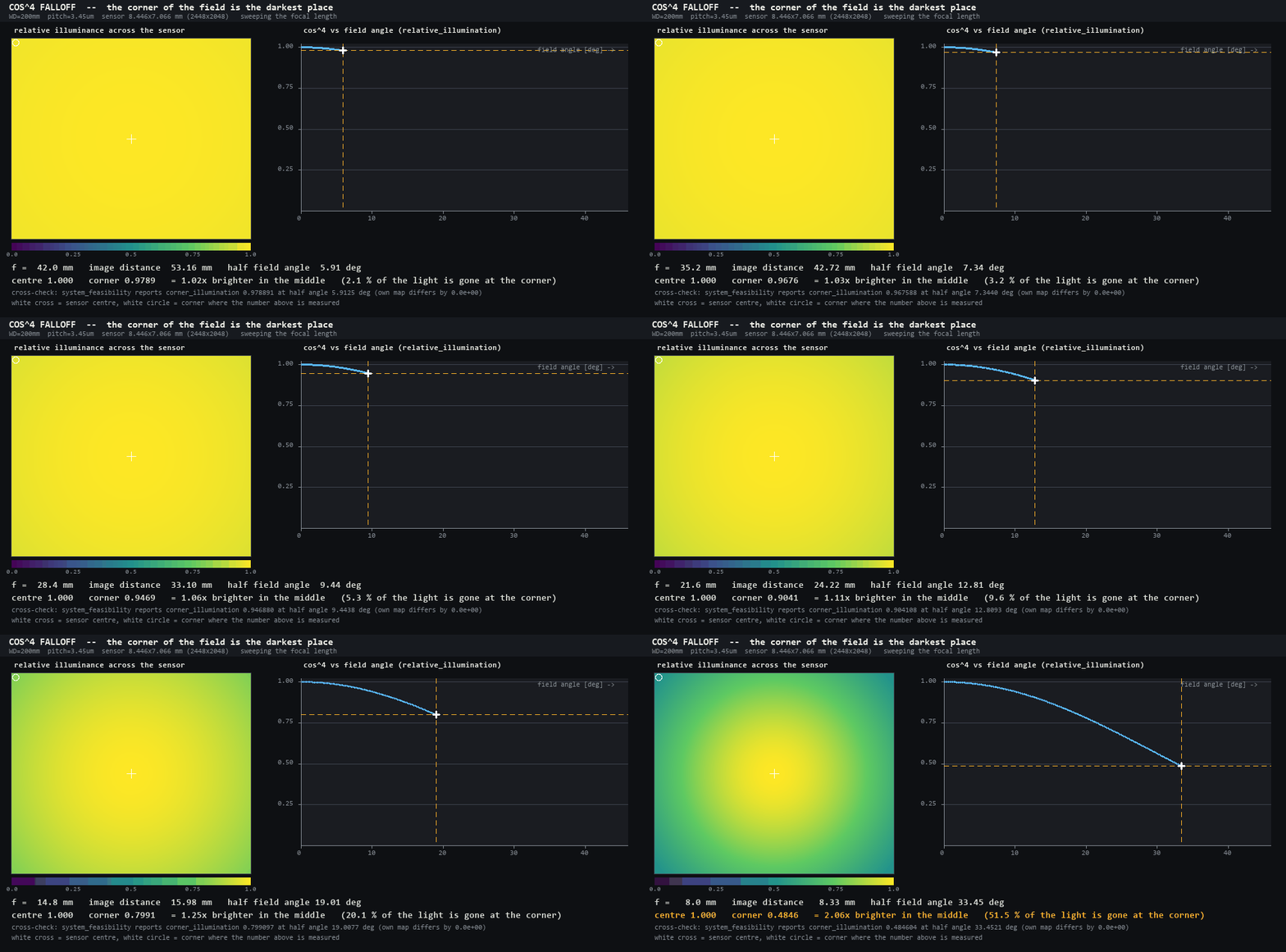
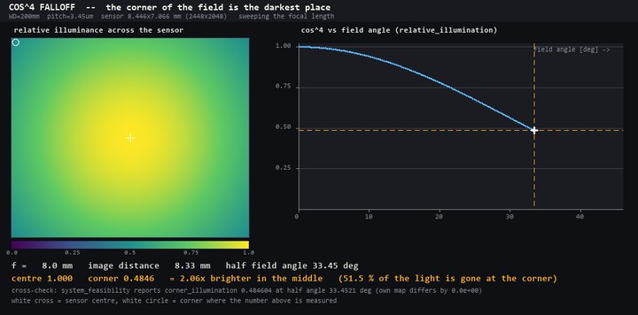
↑ The cos⁴ law of relative illumination — shortening the focal length from 42 to 8 mm widens the half field angle from 5.91° to 33.45°, and the corner of the field darkens to 0.9789 → 0.4846 of the centre. The curve on the right is the raw output of relative_illumination; the map on the left evaluates the same cos⁴ in sensor coordinates — two independent routes whose corner values differ by at most 0.0e+00 (built so that either one breaking would show). Ops used: relative_illumination, thin_lens, system_feasibility, draw_polyline.
A single frame still reads (still thumbnail: wingopt_cos4_falloff_thumb.jpg). 36 frames / 10 fps / 1000×494 px / 1.66 MB.
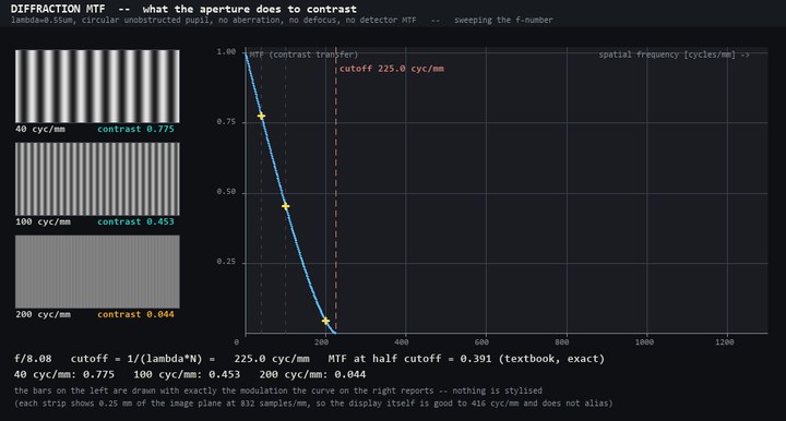
The diffraction-limited MTF
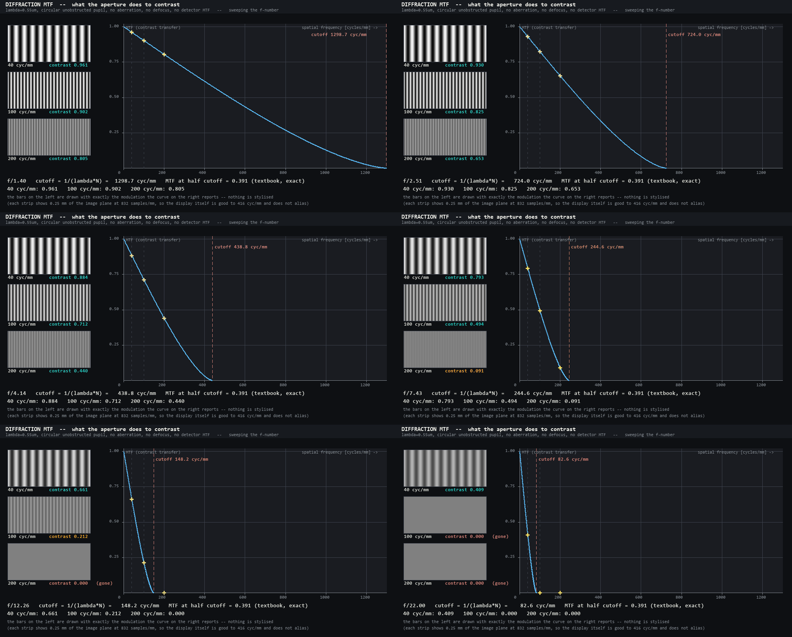
↑ The diffraction-limited MTF — stopping down from f/1.4 to f/22.0 drops the cutoff frequency 1/(λN) from 1299 to 83 cyc/mm. The bars on the left are not decoration: their amplitude is the contrast read straight off the curve on the right, and the 200 cyc/mm bar that stood at 0.805 at f/1.4 is 0.000 at f/22.0 — gone completely. Ops used: mtf_diffraction, draw_polyline, draw_markers.
A single frame still reads (still thumbnail: wingopt_mtf_thumb.jpg). 34 frames / 10 fps / 1000×536 px / 0.99 MB.
Depth of field and the circle of confusion
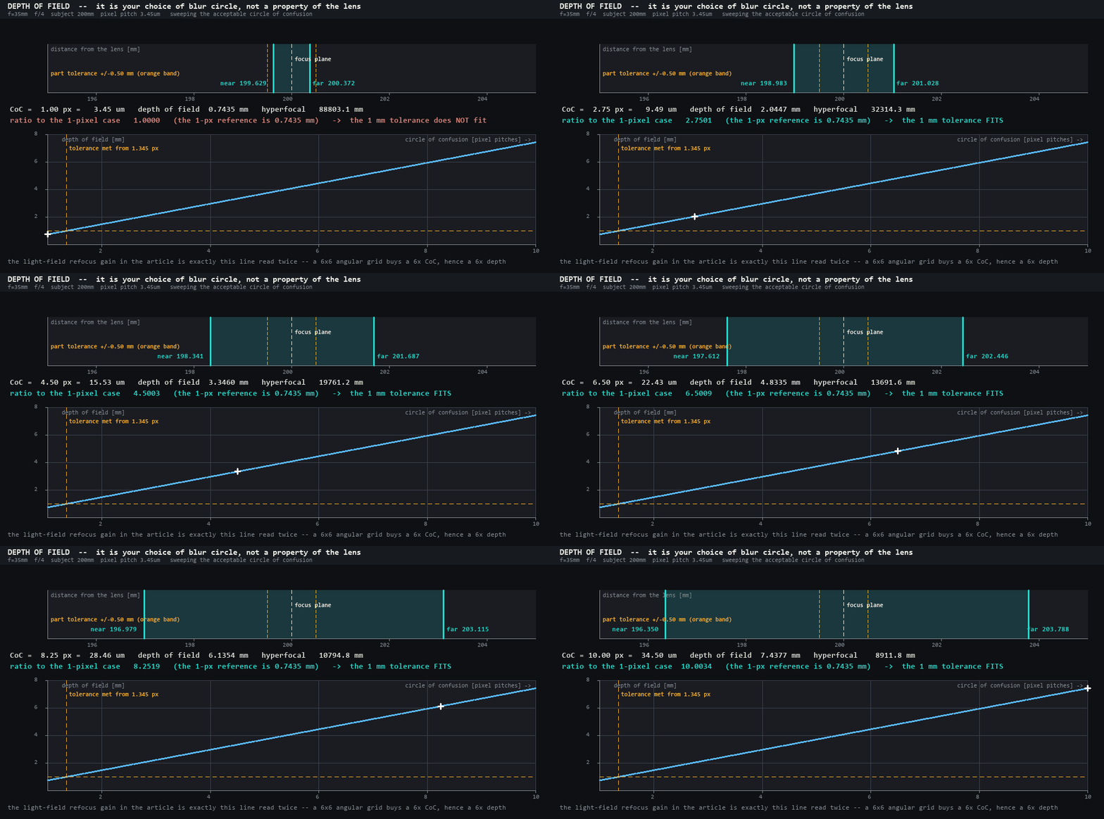
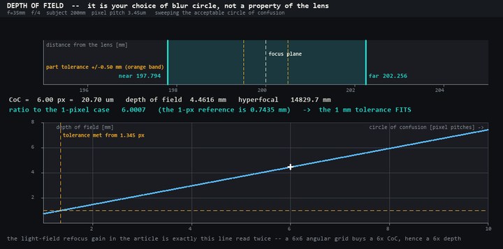
↑ Depth of field and the circle of confusion — depth of field is not a property of the lens; it is a decision you make, namely the acceptable circle of confusion. Widening that circle from 1 pixel to 10 pixels stretches the depth from 0.7435 mm to 7.4377 mm (ratio 10.0034), almost exactly proportionally. The light-field gain table in the article (6.0016x for a 6×6 array) is this same straight line read twice, and the required 1 mm tolerance first fits at a circle of 1.345 pixels. Ops used: depth_of_field, draw_polyline, draw_line.
A single frame still reads (still thumbnail: wingopt_dof_coc_thumb.jpg). 37 frames / 10 fps / 1000×496 px / 0.44 MB.
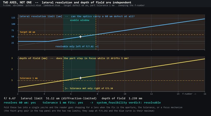
Lateral resolution against depth of field
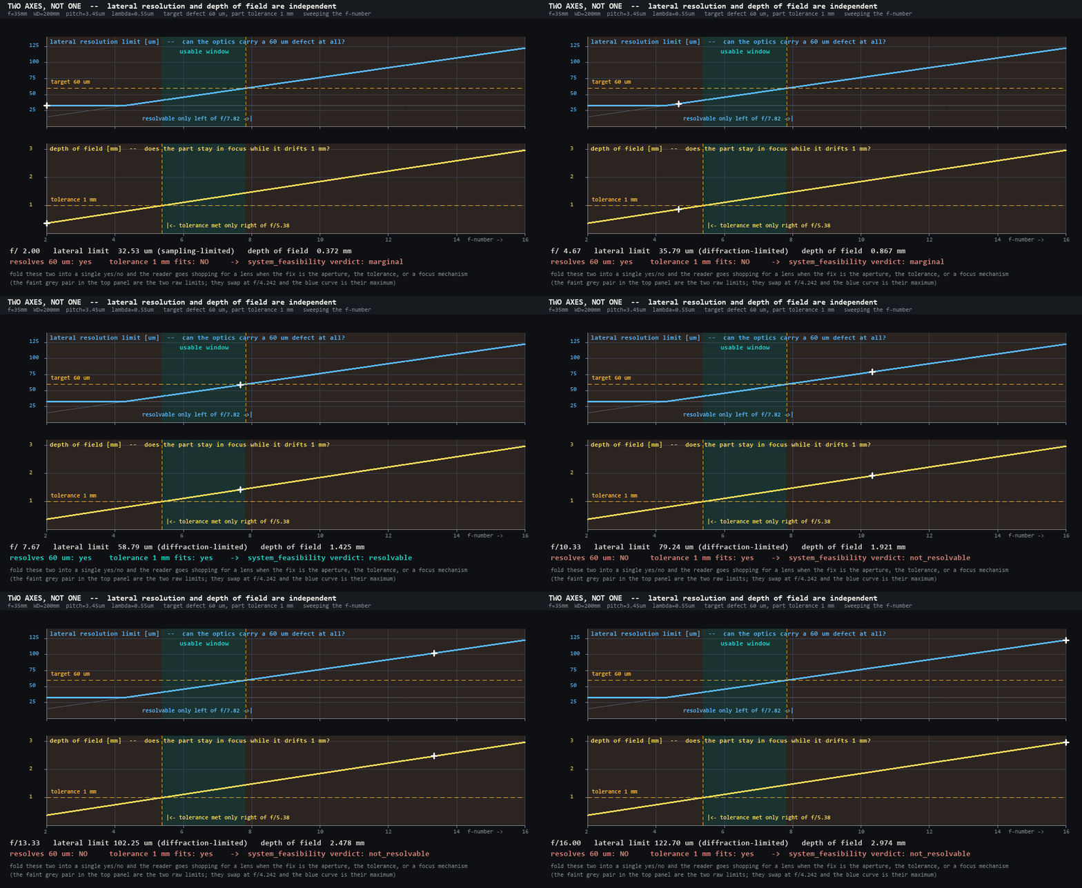
↑ Lateral resolution against depth of field — lateral resolution and depth of field are two independent axes. A 60 µm defect stays resolvable up to f/7.82, while the part’s 1 mm tolerance only fits from f/5.38 — so the usable window is the band f/5.38 to f/7.82 and nothing else. Fold that into a single resolvable flag and it reports “the optical limit was not reached”, at which point the reader goes shopping for a lens (when what needs fixing is the aperture, the tolerance or the focus mechanism). Ops used: resolving_power, depth_of_field, system_geometry, draw_polyline.
A single frame still reads (still thumbnail: wingopt_res_vs_dof_thumb.jpg). 43 frames / 10 fps / 1000×548 px / 0.33 MB.
The Airy pattern and the Rayleigh criterion
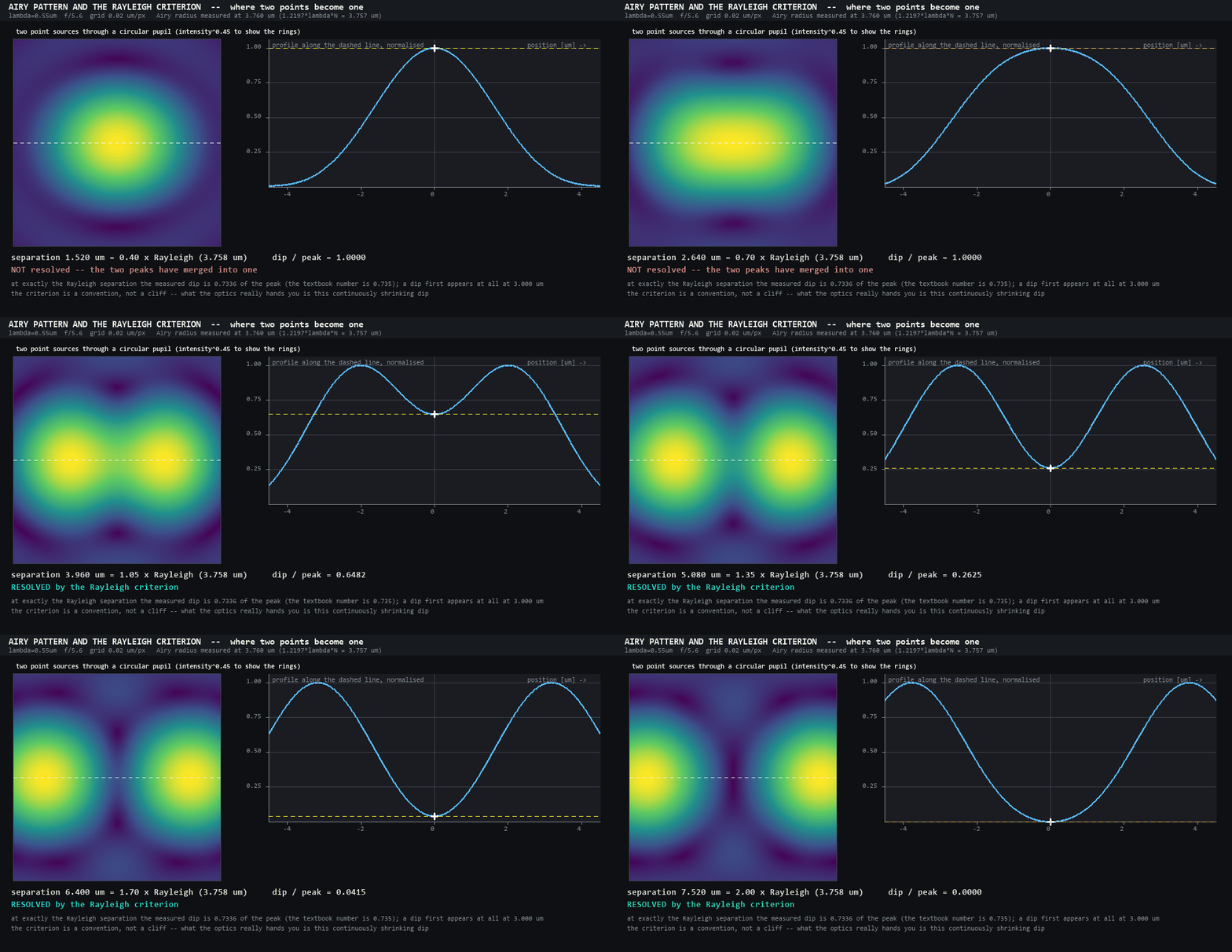
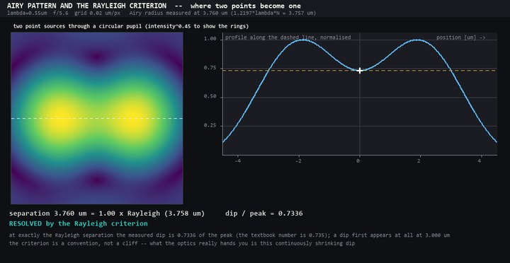
↑ The Airy pattern and the Rayleigh criterion — bring two points together in the Airy image of a circular pupil and the dip between them fills in continuously, not off a cliff. The first dark ring measures 3.760 µm (theory 1.2197λN = 3.757 µm), the dip at the Rayleigh separation of 3.758 µm measures 0.7336 (textbook 0.735), and a dip only begins to appear at all from 3.000 µm. Ops used: airy_pattern, draw_polyline, draw_line.
A single frame still reads (still thumbnail: wingopt_airy_rayleigh_thumb.jpg). 33 frames / 10 fps / 1000×516 px / 2.31 MB.
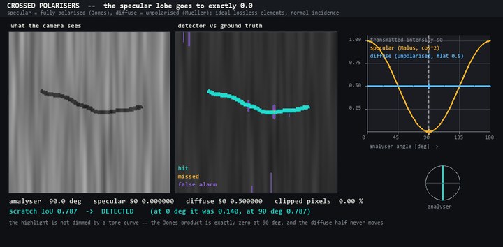
Killing the shine on metal with polarisation
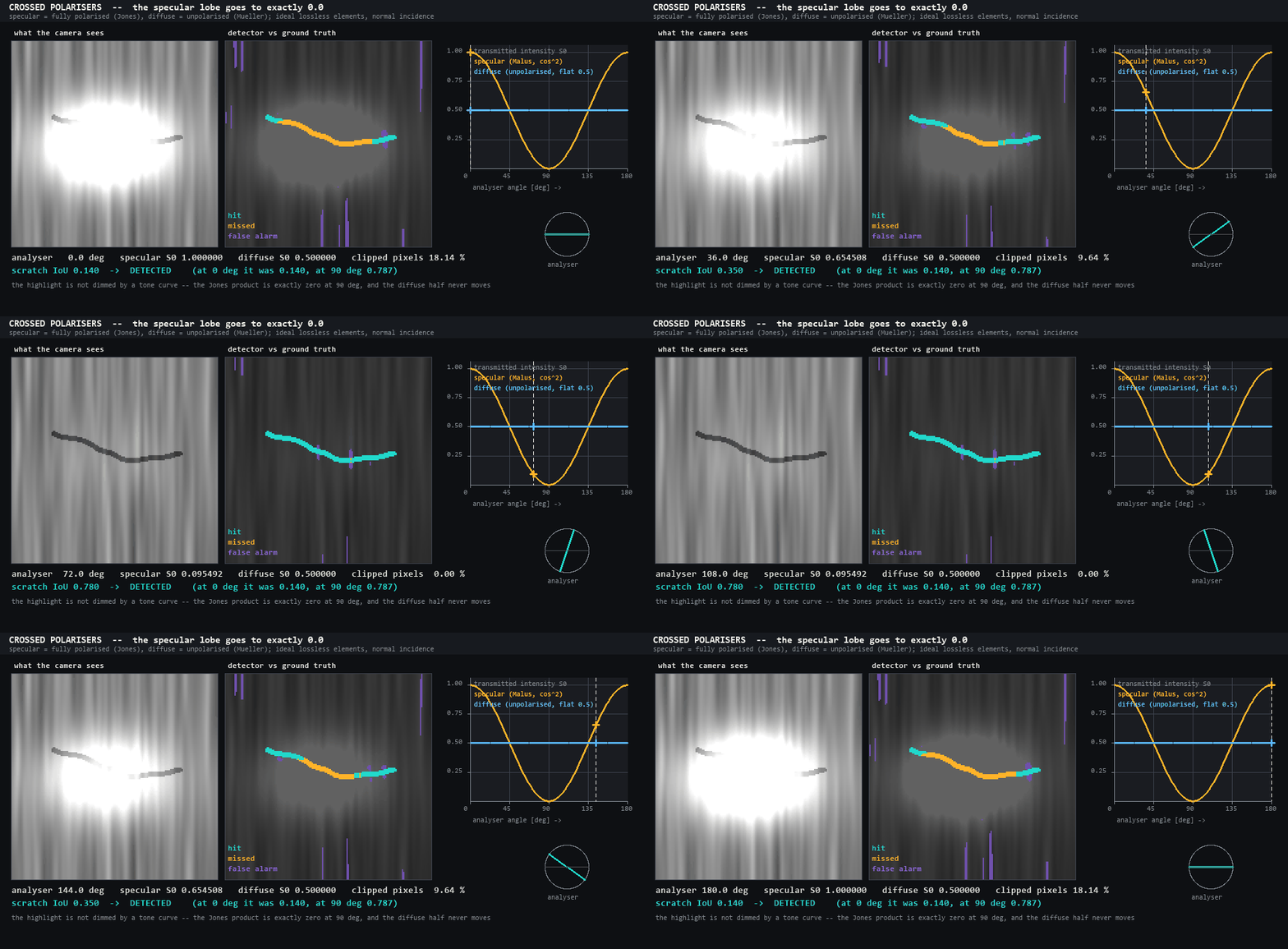
↑ Killing the shine on metal with polarisation — the specular reflection (fully polarised) goes through a Jones matrix, the diffuse reflection (unpolarised) through a Mueller matrix, and the analyser turns from 0° to 180°. By Malus’s law the transmitted specular intensity runs 1.0000 → 0.0000 (exactly 0) while the diffuse component stays at 0.5 regardless of angle — clipped pixels fall from 18.14 % to 0.00 %, and the scratch that was drowning in the glare recovers from an IoU of 0.140 to 0.787, which turns it into a detection. Ops used: jones_element, jones_apply, stokes_from_jones, mueller_element, mueller_apply, defect_scratch, surface_texture, image_formation, draw_circle.
A single frame still reads (still thumbnail: wingopt_polarizer_thumb.jpg). 31 frames / 10 fps / 1000×492 px / 2.65 MB.
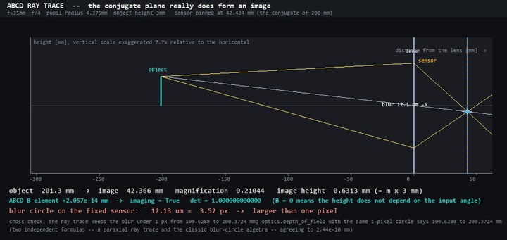
Thin lens / the ABCD matrix
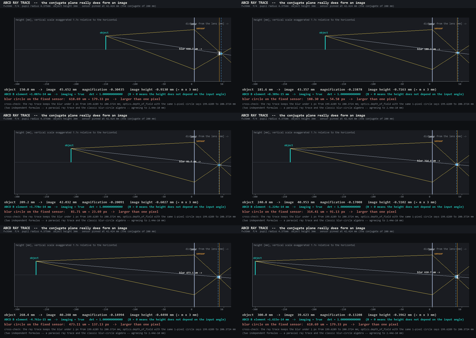
↑ Thin lens / the ABCD matrix — trace three rays through the ABCD matrix while the object distance moves, and at the conjugate plane the B element goes to 0 and the exit height stops depending on the entrance angle — which is the definition of “it is imaging”. The sensor is pinned at 42.424 mm, so the blur circle grows as the object moves back and forth, and the range over which ray tracing says the blur stays within one pixel, 199.6–200.4 mm, agrees with the independent closed form depth_of_field (199.629–200.372 mm) to within the step of the grid. Ops used: abcd_matrix, abcd_trace, thin_lens, depth_of_field, draw_line.
A single frame still reads (still thumbnail: wingopt_abcd_rays_thumb.jpg). 39 frames / 10 fps / 1000×474 px / 0.53 MB.
A map of the detection limit
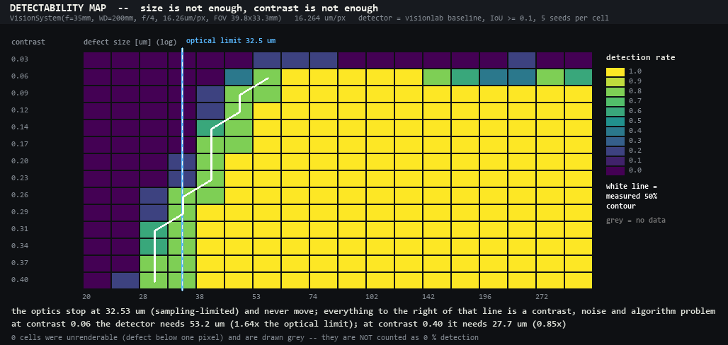
↑ A map of the detection limit — measure the detection rate over the plane of defect size (horizontal, logarithmic) against contrast (vertical) and the optical limit of 32.53 µm (sampling-bound) stands still as a vertical line, while the actual detection boundary (the white line = the measured 50 % contour) moves from 53.2 to 27.7 µm on contrast alone. At a contrast of 0.06 it takes 53 µm (1.64x the limit); raise the contrast to 0.40 and 28 µm (0.85x) is enough — in 4 of the 13 rows the boundary comes out to the left of the limit (detection here is a hit test at IoU ≥ 0.1, not resolution: not “resolved into two separate pixels”). The right-hand side is not a lens problem. Ops used: render_part, system_geometry, resolving_power, draw_polyline, draw_line.
Click for full size (1028×488 px / 40 kB).
What changing the illumination lets you see
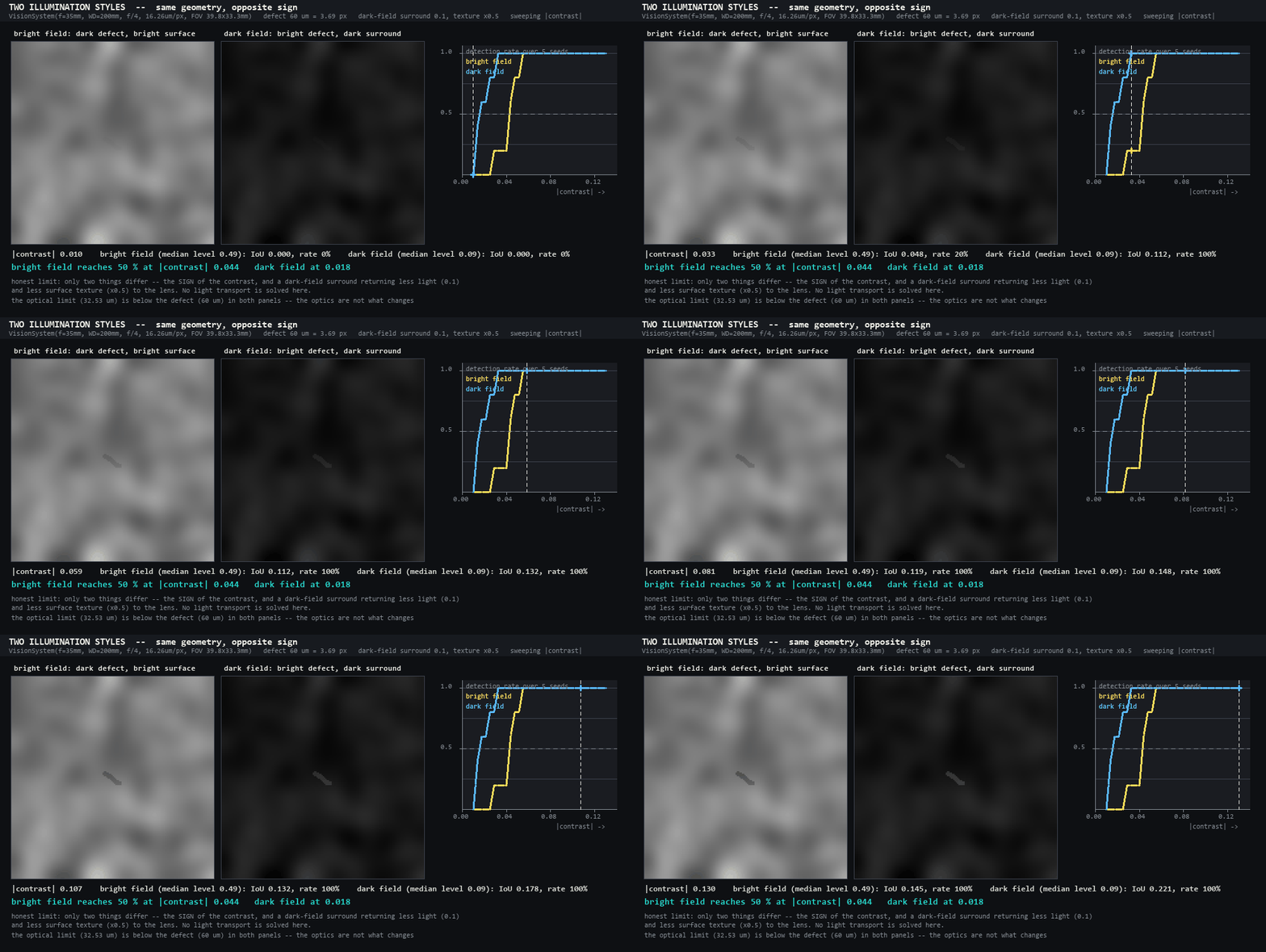
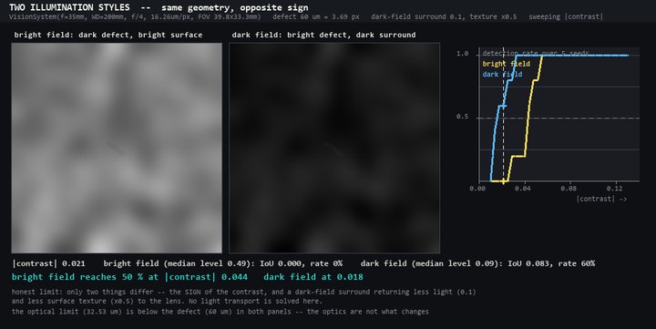
| *↑ What changing the illumination lets you see — the same 60 µm scratch, same geometry, shown bright-field style (a dark scratch on a bright surface) beside dark-field style (a glowing scratch on a dark ground), sweeping the contrast. Bright-field style reaches 50 % detection at | contrast | 0.044, dark-field style at 0.018, and both clear the 32.53 µm optical limit with room to spare — the difference is not the lens, it is the presentation (this is defectgen’s appearance model, that is, a sign and an exposure, not a light-transport calculation for a ring light). Ops used: render_part, defect_scratch, image_formation, draw_polyline.* |
A single frame still reads (still thumbnail: wingopt_illumination_thumb.jpg). 33 frames / 10 fps / 1000×502 px / 0.30 MB.
Pixel pitch and sampling
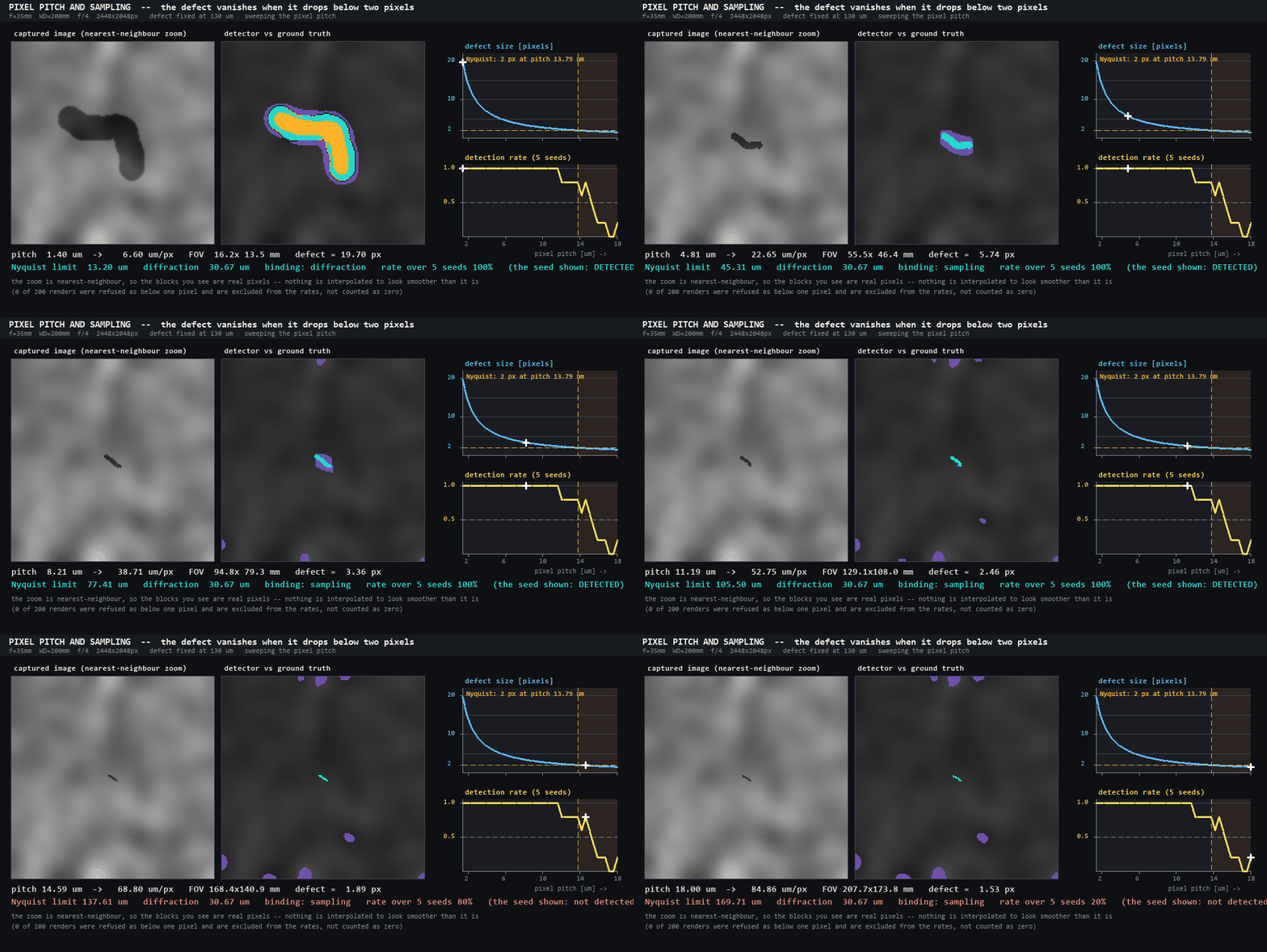
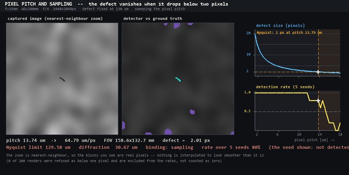
↑ Pixel pitch and sampling — hold a 130 µm scratch fixed and coarsen only the pixel pitch: the defect drops below 2 pixels at a pitch of 13.79 µm (the Nyquist boundary), while measured 50 % detection survives to a pitch of 15.02 µm. The zoom is nearest-neighbour, so the squares you see are the real pixels — no interpolation was added to make them look smooth. Ops used: render_part, system_geometry, resolving_power, draw_polyline.
A single frame still reads (still thumbnail: wingopt_pixel_pitch_thumb.jpg). 40 frames / 10 fps / 1000×502 px / 0.58 MB.
The generated files (measured)
| Exhibit | Format | Pixels | Frames | Size | SHA-256 (first 16) |
|---|---|---|---|---|---|
| The one road from design to verdict | GIF | 940×514 | 6 | 303 kB | 46c1de110827b53c |
| A sample book of the defect generator | PNG | 998×882 | 1 | 146 kB | c732c5100726f75c |
| The limits change places | GIF | 1000×474 | 42 | 459 kB | 353cbabaa24686ab |
| The cos⁴ law of relative illumination | GIF | 1000×494 | 36 | 1661 kB | 50142cb5931e55a0 |
| The diffraction-limited MTF | GIF | 1000×536 | 34 | 991 kB | b52ec1dd5cf66bd8 |
| Depth of field and the circle of confusion | GIF | 1000×496 | 37 | 439 kB | 0f2b9c69b1bb6dc5 |
| Lateral resolution against depth of field | GIF | 1000×548 | 43 | 327 kB | b89bed20b13b8978 |
| The Airy pattern and the Rayleigh criterion | GIF | 1000×516 | 33 | 2312 kB | 5d8a032aef0b8560 |
| Killing the shine on metal with polarisation | GIF | 1000×492 | 31 | 2651 kB | 7201c5f510b43e36 |
| Thin lens / the ABCD matrix | GIF | 1000×474 | 39 | 533 kB | 9b69c483a02265f2 |
| A map of the detection limit | PNG | 1028×488 | 1 | 40 kB | 81b870b0b2bbbd90 |
| What changing the illumination lets you see | GIF | 1000×502 | 33 | 297 kB | 9de5ff51d03720e0 |
| Pixel pitch and sampling | GIF | 1000×502 | 40 | 577 kB | 54e2158fdb88a94a |